
You can use the formula bar to edit the contents of a selected cell, or you can perform your editing “on location” in the cell. Excel 2010 also includes a few special features you can apply to tasks such as entering date sequences, which once involved editing each cell but are now semiautomatic, if you know where to find the “trigger.”
While typing or editing the contents of a cell, you can use Cut, Copy, Paste, and Clear to manipulate cell entries. Often, retyping a value or formula is easier, but using commands is convenient when you’re working with long, complex formulas or with labels. When you’re working in a cell or in the formula bar, these commands work just as they do in a word-processing program such as Word. For example, you can copy all or part of a formula from one cell to another. For example, suppose cell A10 contains the formula =IF(NPV(.15,A1:A9)>0,A11,A12) and you want to type =NPV(.15,A1:A9) in cell B10.
Note
You can edit the contents of cells without using the formula bar. By double-clicking a cell, you can perform any formula bar editing procedure directly in the cell.

To do so, select cell A10, and in the formula bar, select the characters you want to copy—in this case, NPV(.15,A1:A9). Then press Ctrl+C, or click the Copy button (located in the Clipboard group on the Home tab). Finally, select cell B10, type = to begin a formula, and press Ctrl+V (or click the Paste button).
Note
Excel does not adjust cell references when you cut, copy, and paste within a cell or in the formula bar. For information about adjustable references, see How Copying Affects Cell References on page 472.
When you type or edit formulas containing references, Excel gives you visual aids called range finders to help you audit, as shown in Figure 8-19, where we obviously have a problem with our SUM formula. The total should include all the rows of data, so drag a handle on a bottom corner of the range selection rectangle until it includes all the correct cells.

Note
For more information about formulas, see Chapter 12. For more about auditing, see Auditing and Documenting Worksheets on page 261.
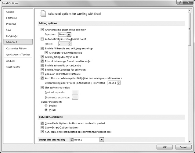
The Advanced category in the Excel Options dialog box (click the File tab and then Options) contains an assortment of options that control editing-related workspace settings, as shown in Figure 8-20. These options include the following:
After Pressing Enter, Move Selection This locks in the entry and makes the cell below active. To change the direction of the selection after you press Enter, use the Direction drop-down list. When you clear this check box, pressing Enter locks in the entry and leaves the same cell active.
Automatically Insert A Decimal Point For those of us who remember using 10-key calculators, this is equivalent to the “floating point” setting. Ordinarily you type numbers and decimal points manually. To have Excel enter decimal points for you, select this option, and then select the number of decimal places you want. For example, when you type 12345 with two decimal places specified, Excel enters 123.45 in the cell. When you apply this option, Fixed Decimal appears in the status bar. This option applies only to entries you make after you select it, without altering existing data. It also applies only when you do not type a decimal point. If you type a number including a decimal point, the option has no effect.
Enable Fill Handle And Cell Drag-And-Drop This is required for the direct manipulation of cells using the mouse. See Moving and Copying with the Mouse on page 210. Leaving the Alert Before Overwriting Cells option selected is always a good idea.
Allow Editing Directly In Cells This is required for in-cell editing. See Editing in Cells or in the Formula Bar on page 225.
Extend Data Range Formats And Formulas This lets Excel apply formatting from existing cells to new cells entered in a list or table. See Extending Existing Formatting on page 238.
Enable Automatic Percent Entry This helps you type values in cells with the Percentage format. When you select this check box, all entries less than 1 are multiplied by 100. When you clear this check box, all entries—including those greater than 1—are multiplied by 100. For example, in a cell to which you have already applied the Percentage format, typing either .9 or 90 produces the same result—90%—in the cell. If you clear the Enable Automatic Percent Entry check box, typing 90 results in the displayed value 9000% (as long as you have applied the Percentage format to the cell).
Enable AutoComplete For Cell Values This lets Excel suggest cell entries by comparing existing values it finds in the same column as you type. See Letting Excel Help with Typing Chores on page 249.
Zoom On Roll With IntelliMouse Ordinarily, if your mouse has a wheel, rotating it causes the worksheet to scroll (or zoom while pressing Ctrl). Select this check box to switch the behavior of the wheel so that the worksheet zooms when you rotate the wheel (or scrolls while you press Ctrl).
Alert The User When A Potentially Time-Consuming Operation Occurs If an editing operation will affect a large number of cells, this option controls whether you are notified and lets you specify the number of cells it takes to trigger the notification.
Use System Separators Ordinarily Excel defaults to the designated numeric separators for decimals and thousands (periods and commas, respectively) specified by your Windows system settings. If you want to specify alternative separators, you can do so here.
Show Paste Options Button/Show Insert Options Buttons This activates the floating button menus that appear after pasting or inserting. Ordinarily, after you perform a paste or an insert operation, a floating button appears, offering a menu of various context-specific actions you can then perform. Clear these options to turn off these features.
Cut, Copy, And Sort Inserted Objects With Their Parent Cells This is required to “attach” graphic objects to cells. See Tools to Help You Position Objects on the Worksheet on page 428.
As described earlier in this chapter, the fill handle has many talents to make it simple to enter data in worksheets. Uses of the fill handle include quickly and easily filling cells and creating data series by using the incredibly useful Auto Fill feature.
Take a look at Figure 8-21. If you select cell B2 in this worksheet and drag the fill handle down to cell B5, Excel copies the contents of cell B2 to cells B3 through B5. However, if you click the floating Auto Fill Options button that appears after you drag, you can select a different Auto Fill action, as shown in Figure 8-22.


Figure 8-22. Create a simple series by dragging the fill handle and then clicking Fill Series on the Auto Fill Options menu.
Tip
INSIDE OUT Create Decreasing Series
Generally, when you create a series, you drag the fill handle down or to the right, and the values increase accordingly. You can also create a series of decreasing values by dragging the fill handle up or to the left. Select the starting values in cells at the bottom or to the right of the range you want to fill, and then drag the fill handle back toward the beginning of the range.
If you click Fill Series on the Auto Fill Options menu, Excel creates the simple series 21, 22, and 23 instead of copying the contents of cell C2. If, instead of selecting a single cell, you select the range C1:C2 in Figure 8-22 and drag the fill handle down to cell C5, you create a series that is based on the interval between the two selected values, resulting in the series 30, 40, and 50 in cells C3:C5. If you click Copy Cells on the Auto Fill Options menu, Excel copies the cells instead of extending the series, repeating the pattern of selected cells as necessary to fill the range. Instead of filling C3:C5 with the values 30, 40, and 50, choosing Copy Cells will enter the values 10, 20, and 10 in C3:C5.
If you select a text value and drag the fill handle, Excel copies the text to the cells where you drag. If, however, the selection contains both text and numeric values, the Auto Fill feature takes over and extends the numeric component while copying the text component. You can also extend dates in this way, using a number of date formats, including Qtr 1, Qtr 2, and so on. If you type text that describes dates, even without numbers (such as months or days of the week), Excel treats the text as a series.
Tip
INSIDE OUT Fill Series Limited to 255 Characters
Excel lets you type up to 32,767 characters in a cell. However, if you want to extend a series using Auto Fill, the selected source cells cannot contain more than 255 characters. If you try to extend a series from an entry of 256 characters or more, Excel copies the cells instead of extending the series. This is not really a bug but a side effect of the Excel column-width limitation of 255 characters. Besides, a 256-character entry is not going to be readable on the screen anyway. If you really need to create a series out of humongous cell entries like this, perhaps a little worksheet redesign is in order. Otherwise, you have to do it manually.
Figure 8-23 shows some examples of simple data series created by selecting single cells containing values and dragging the fill handle. We typed the values in column A, and we extended the values to the right of column A using the fill handle. Figure 8-24 shows examples of creating data series using two selected values that, in effect, specify the interval to be used in creating the data series. We typed the values in columns A and B and extended the values to the right of column B using the fill handle. These two figures also show how Auto Fill can create a series even when you mix text and numeric values in cells. Also note that we extended the values and series in Figure 8-24 by selecting the entire range of starting values in cells A3:B12 before dragging the fill handle to extend them, showing how Excel can extend multiple series at once. (We applied the bold formatting after filling to make it easier to differentiate the starting values.)
Note
If you select more than one cell and hold down Ctrl while dragging the fill handle, you suppress Auto Fill and copy the selected values to the adjacent cells. Conversely, with a single value selected, holding down Ctrl and dragging the fill handle extends a series, contrary to the regular behavior of copying the cell.


Figure 8-24. Specify data series intervals by selecting a range of values and dragging the fill handle.
Sometimes you can double-click the fill handle to extend a series from a selected range. Auto Fill determines the size of the range by matching an adjacent range. For example, in Figure 8-25, we filled column A with a series of values. Then we filled column B by selecting the range B1:B2 and double-clicking the fill handle. The newly created series stops at cell B5 to match the adjacent cells in column A. When the selected cells contain something other than a series, such as simple text entries, double-clicking the fill handle copies the selected cells down to match the length of the adjacent range.

Figure 8-25. We extended a series into B3:B5 by selecting B1:B2 and double-clicking the fill handle.
Tip
INSIDE OUT How Auto Fill Handles Dates and Times
Auto Fill ordinarily increments recognizable date and time values when you drag the fill handle, even if you initially select only one cell. For example, if you select a cell that contains Qtr 1 or 1/1/2011 and drag the fill handle, Auto Fill extends the series as Qtr 2, Qtr 3, or 1/2/2011, 1/3/2011, and so on. If you click the Auto Fill Options menu after you drag, you’ll see that special options become available if the original selection contains dates or the names of days or months:

An interesting feature of this menu is Fill Weekdays, which not only increments a day or date series but also skips weekend days. Depending on the original selection, different options might be available on the menu.
When you use the right mouse button to fill a range or extend a series, a shortcut menu appears when you release the button, as shown in Figure 8-26. This menu differs somewhat from the Auto Fill Options menu and lets you specify what you want to happen in advance, as opposed to the Auto Fill Options menu giving you the ability to change the action after the fact.
The box that appears on the screen adjacent to the pointer indicates what the last number of this sequence would be if we dragged the fill handle as usual (with the left mouse button)—in this case, 160. The Linear Trend command creates a simple linear series similar to that which you can create by dragging the fill handle with the left mouse button. Growth Trend creates a simple nonlinear growth series by using the selected cells to extrapolate points along an exponential growth curve. In Figure 8-27, rows 4 through 6 in column A contain a series created using Linear Trend, and the same rows in column C contain a series created using Growth Trend, starting with the same values.


Clicking the Series command on the Home tab, Editing Group, Fill menu displays the Series dialog box shown in Figure 8-28, letting you create custom incremental series. Alternatively, you can display the Series dialog box by selecting one or more cells containing numbers, dragging the fill handle with the right mouse button, and clicking Series on the shortcut menu.

In the Series dialog box you can specify an interval with which to increment the series (step value) and a maximum value for the series (stop value). Using this method has a couple of advantages over direct mouse manipulation techniques. First, you do not need to select a range to fill, and second, you can specify increments (step values) without first selecting cells containing examples of incremented values. You can select examples of values if you want, but it is not necessary.
The Rows option tells Excel to use the first value in each row to fill the cells to the right. The Columns option tells Excel to use the first value in each column to fill the cells below. For example, if you select a range of cells in advance that is taller than it is wide, Excel automatically selects the Columns option when you open the Series dialog box. Excel uses the Type options in conjunction with the start values in selected cells and the value in the Step Value box to create your series. If you select examples first, Step Value reflects the increment between the selected cells.
The Linear option adds the value specified in the Step Value box to the selected values in your worksheet to extend the series. The Growth option multiplies the last value in the selection by the step value and extrapolates the rest of the values to create the series. If you select the Date option, you can specify the type of date series from the options in the Date Unit area. The Auto Fill option works like using the fill handle to drag a series, extending the series by using the interval between the selected values; it determines the type of data and attempts to “divine” your intention. Selecting the Trend check box extrapolates an exponential series, but it works only if you select more than one value before displaying the Series dialog box.
Note
For more about typing dates, see Entering a Series of Dates on page 568.
Use the Down, Right, Up, and Left commands on the Fill menu, shown in Figure 8-29, to copy selected cells to an adjacent range of cells. Before clicking these commands, select the range you want to fill, including the cell or cells containing the formulas, values, and formats you want to use to fill the selected range. (Comments are not included when you use these Fill commands.)
Suppose cell A1 contains the value 100. In Figure 8-29, we selected the range A1:K2 and then clicked Fill, Right to copy the value 100 across row 1. With the range still selected, we can click Fill, Down to finish filling the selected range with the original value.
Note
You can also use keyboard shortcuts to duplicate Home, Fill, Down (press Ctrl+D) and Home, Fill, Right (press Ctrl+R).

The Across Worksheets command on the Fill menu copies cells from one worksheet to other worksheets in the same workbook. For more information about using the Across Worksheets command, see Filling a Group on page 260.
Clicking Fill, Justify doesn’t do what you might think it does. It splits a cell entry and distributes it into two or more adjacent rows. Unlike other Fill commands, Justify modifies the contents of the original cell.
Note
For information about the other justify feature—that is, justifying text in a single cell—see “Justifying Text in Cells” on page 346.
For example, in the worksheet on the left in Figure 8-30, cell A1 contains a long text entry. To divide this text into cell-sized parts, select cell A1, and click Home, Fill, Justify. The result appears on the right in Figure 8-30.

When you click Justify, Excel displays a message warning you that this command uses as many cells below the selection as necessary to distribute the contents. Excel overwrites any cells that are in the way in the following manner:
If you select a multirow range, Justify redistributes the text in all selected cells. For example, you can widen column A in Figure 8-30, select the filled range A1:A6, and click Justify again to redistribute the contents using the new column width.
If you select a multicolumn range, Justify redistributes only the entries in the leftmost column of the range, but it uses the total width of the range you select as its guideline for determining the length of the justified text. The cells in adjacent columns are not affected, although the justified text appears truncated if the adjacent column’s cells are not empty.
If you find yourself repeatedly entering a particular sequence in your worksheets, such as a list of names or products, you can use the Excel Custom Lists feature to make entering that sequence as easy as dragging the mouse. After you create your custom list, you can enter it into any range of cells by typing any item from the sequence in a cell and then dragging the fill handle. For example, in Figure 8-31 we entered a single name in cell A1 and dragged the fill handle down. The text in cells A2:A9 was filled in automatically matching the sequence in the custom list we created.
To create a custom list, follow these steps:
Click the File tab, click Options, and click the Advanced category.
Scroll all the way to the bottom, and click the Edit Custom Lists button (under General).
With New List selected in the Custom Lists box, type the items you want to include in your list in the List Entries box. Be sure to type the items in the order you want them to appear.
Click OK to return to the worksheet.

You can also create a custom list by importing the entries in an existing cell range. To import the entries shown in Figure 8-31, we selected a cell range containing the list of names before opening the Excel Options dialog box. When you open the Edit Custom Lists dialog box, the address of the selected range appears next to the Import button, which you can click to add the new list. (You can also select the list after opening the dialog box. You need to click in the edit box next to the Import button, and then you can drag on the worksheet to select the cells.)
Excel has several AutoFormat features designed to help speed things up as you work. The format-extension feature lets you add new rows and columns of data to a previously constructed table without having to apply formatting to the new cells—theoretically, at least. For example, if you want to add another column to the existing table in Figure 8-32, select cell E3, type the column heading, and then continue entering numbers in cells E4–E7. Excel surmises that you want the new entries to use the same formatting as the adjacent cells above or to the left and picks up their cell and text formats.

Figure 8-32. Automatic format extension helps apply formatting to new cells, but it goes only so far.
However, as you can see in Figure 8-32, border formats are not picked up, and the feature does not work when entering formulas, as in cells E8 and E9. To be fair, it would make more sense to select the formulas in D8:D9 and drag the fill handle to the right, which would copy the formats, too. So, the format-extension feature does help, but expect to do some cleanup. You can turn this feature off by clicking the File tab, clicking Options, and then in the Advanced category clearing the Extend Data Range Formats And Formulas check box.
Tables are another feature with special AutoFormat qualities. If you are working with a table, additional options control the extension of formatting and formulas. Click the File tab, click Options, and then select the Proofing category. Click the AutoCorrect Options button to display the AutoCorrect dialog box shown in Figure 8-33. The tab labeled AutoFormat As You Type contains the pertinent options.

Figure 8-33. The AutoCorrect dialog box controls automatic format and formula extension when working in tables.
As you can see in Figure 8-33, the AutoFormat As You Type tab includes two options pertaining to tables and one that controls whether Excel automatically creates hyperlinks whenever you type recognizable Internet and network paths. This is very handy if you want to include one-click access to supporting information in your worksheets—or very annoying if you don’t.
Note
For more about AutoCorrect, see Fixing Errors as You Type on page 246. For more about tables, see Chapter 22.