
Excel 2010 provides a rich set of options for formatting the background areas of your charts—including the plot area, the chart area, and the walls and floors of three-dimensional charts. You can also apply these formatting options to legends, to the background areas of titles and data labels, and to certain kinds of chart markers—including columns, bars, pyramids, cones, cylinders, areas, bubbles, pie slices, and doughnut bites.
To format a chart element’s area, double-click the element. The area-formatting options for a selected chart item appear when you select Fill in the item’s formatting dialog box. Figure 21-3 shows the Fill options for the Format Plot Area dialog box. As for line formatting, the default option for area formatting is Automatic, which means “let Excel decide.”
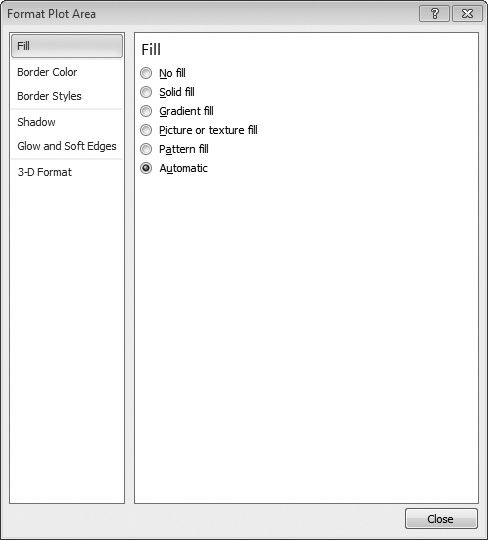
Figure 21-3. Click Fill in the Format Chart Area dialog box to apply solid colors, gradients, pictures, and textures to background areas of your charts.
A default chart displayed on a white worksheet has a solid white background. Note that this is not the same as having no fill; a chart area with no fill is transparent, which allows the underlying worksheet gridlines to shine through.
Making the chart area transparent can be useful at times. If you want to create a worksheet display that minimizes the chart apparatus and simply shows a small graphic to support a set of numbers, using the No Fill option is good way to get there. (A sparkline can serve this purpose as well, of course, but sparklines, described in the previous chapter, are available only in a small number of chart types.) Eliminate the border around the chart area (see Formatting Lines and Borders on page 699), get rid of any chart elements you don’t want (the title, legend, or whatever), and assign the No Fill option to your chart and plot areas. Figure 21-4 shows an example of a chart reduced to basics in this way.

A color gradient is a smooth progression of color tones from one part of an area to another—for example, a transition from bright red at the top of a column marker to black at the bottom. Color gradients can give your chart areas a classy, professional appearance. Of course, depending on how you use them, color gradients can also be distracting. If you’re creating charts that are intended to convince or impress others, it’s probably a good idea to exercise a bit of restraint in using gradients. On the other hand, if flamboyance is your style, Excel gives you plenty of ways to express yourself.
Figure 21-5 shows the Fill category of the Format Chart Area dialog box with the Gradient Fill option selected. The options presented here can be a little bewildering at first. Fortunately, the Excel 2010 Live Preview capability lets you see the effect of a setting on your chart before you leave the dialog box. Experiment on a large region of a chart, such as the plot area of a chart you’ve moved to a chart sheet, and you’ll quickly get an idea of what’s possible.

Figure 21-5. The Excel 2010 Gradient Fill options let you select colors, angles, directions, transparency, and more.
A good way to begin your exploration is to open the Preset Colors drop-down list:

The Preset Colors gallery offers two dozen attractive color gradients. In the gallery, the gradients are all of the same type and direction (moving in a linear fashion from top to bottom), but you can apply other type and direction options to them. Choose one, then choose one of the Direction options, open the Direction drop-down list, and you’ll see another gallery that looks like this (for the Linear type):

You don’t have to stick with the 24 options under Preset Colors, of course. With the Gradient Stops, Color, Stop Position, and Transparency controls, you can create any kind of gradient that suits you. Gradient stops are boundaries between colors. You can have as many stops and colors as you want. The Stop Position slider determines where the stop occurs; to add a new stop, click on the slider. If you want, you can add a degree of transparency to any or all sections of your gradient.
If you don’t care for solids or gradients, why not fill your background areas or data markers with textures or pictures? You can use images in a wide variety of supported formats, paste an item from your clip art library (or from Microsoft Office Online), or use one of the 24 texture images supplied by Excel. The latter evoke familiar materials, such as oak, marble, and cloth. For example, Figure 21-6 shows a fish-fossil texture applied to a chart’s plot area, with a clip art image applied to the column markers.
To apply a texture or picture, click Picture Or Texture Fill in the format dialog box for the chart element you have selected. Open the Texture drop-down list to choose from the texture gallery, or click the File, Clipboard, or ClipArt buttons to apply a picture. Excel stretches pictures to fit unless you also select the Tile Picture As Texture check box. If you’re using a bitmapped image, the stretching is likely to produce distortion unless the size of the picture is exactly that of the area you’re formatting. To avoid distortion, you can shrink the image by moving it away from the left, right, top, and bottom borders of the area—in other words, by setting margins. To do that, set nonzero values in the various Offset text boxes.
If you choose to tile the picture, you get a different set of scaling and offset options. You can also create some interesting mirror effects by experimenting with the Mirror Type drop-down list.
