
As you will see, there are many ways beyond a simple click-and-drag to isolate the particular types of data, formats, objects, and even blank cells that you need to gather or edit. Here are a few pertinent facts and definitions to start with:
While a region is defined as a rectangular block of filled cells, a range is any rectangle of cells, filled or empty.
Before you can work with a cell or range, you must select it, and when you do, it becomes active.
The reference of the active cell appears in the Name box at the left end of the formula bar.
You can select ranges of cells, but only one cell can be active at a time. The active cell always starts in the upper-left corner of the range, but you can move it without changing the selection.
Select all cells on a worksheet by clicking the Select All box located in the upper-left corner of your worksheet, where the column and row headings intersect.
For more about selection, read on.
To select a range of cells, drag the mouse over the range. Or, select a cell at one corner, then press Shift and click the cell at the diagonal corner of the range. For example, with cells A1:B5 selected, hold down the Shift key and click cell C10 to select A1:C10. When you need to select a large range, this technique is more efficient than dragging the mouse across the entire selection.
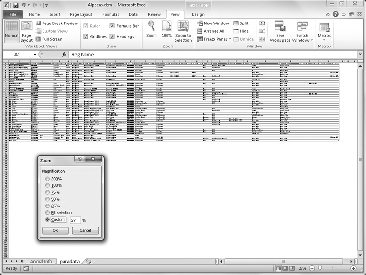
You can zoom out for a bird’s-eye view of a large worksheet, as shown in Figure 6-2. Drag the Zoom slider at the bottom of the screen to the left, or click the Zoom percentage indicator adjacent to the slider to open the Zoom dialog box for more zooming options. The Zoom feature is limited to a range from 10 through 400 percent.
A nonadjacent range (also known as multiple or noncontiguous) comprises more than one selection rectangle, as shown in Figure 6-3. To select multiple ranges with the mouse, press the Ctrl key, and drag through each range you want to select. The first cell you click in the last range you select becomes the active cell. As you can see in Figure 6-3, cell G6 is the active cell.

Use the following methods to select with the mouse:
To select an entire column or row, click the column or row heading. The first visible cell in the column becomes the active cell. If the first row visible on your screen is row 1000, then cell A1000 becomes active when you click the heading for column A, even though all the other cells in the column are selected.
To select more than one adjacent column or row at a time, drag through the column or row headings, or click the heading at one end of the range, press Shift, and then click the heading at the other end.
To select nonadjacent columns or rows, hold down Ctrl, and click each heading or drag through adjacent headings you want to select.
In Figure 6-4, we clicked the heading in column A, then pressed Ctrl while dragging through the headings for rows 1, 2, and 3.

Figure 6-4. Select entire columns and rows by clicking their headings, or hold down the Ctrl key while clicking to select nonadjacent rows and columns.
Use the following methods to select with the keyboard:
To select an entire column with the keyboard, select any cell in the column, and press Ctrl+Spacebar.
To select an entire row with the keyboard, select any cell in the row, and press Shift+Spacebar.
To select several entire adjacent columns or rows with the keyboard, select any cell range that includes cells in each of the columns or rows, and then press Ctrl+Spacebar or Shift+Spacebar, respectively. For example, to select columns B, C, and D, select B4:D4 (or any range that includes cells in these three columns), and then press Ctrl+Spacebar.
To select the entire worksheet with the keyboard, press Ctrl+Shift+Spacebar.
If you hold down the Shift key while navigating regions (as described in Navigating Regions with the Keyboard on page 138), Excel selects all the cells in between. For example, if cell A3 was the only cell selected in the worksheet shown in Figure 6-4, pressing Ctrl+Right Arrow would select the range A3:E3, and then pressing Ctrl+Down Arrow would select the range A3:E7.
At the right end of the Home tab on the ribbon, the Find & Select menu displays several helpful selection commands, as shown in Figure 6-5. In the middle of the menu are five commands that used to be buried in dialog boxes back in the old days, but they’ve more recently been promoted to the ribbon because of their widespread use: Formulas, Comments, Conditional Formatting, Constants, and Data Validation.
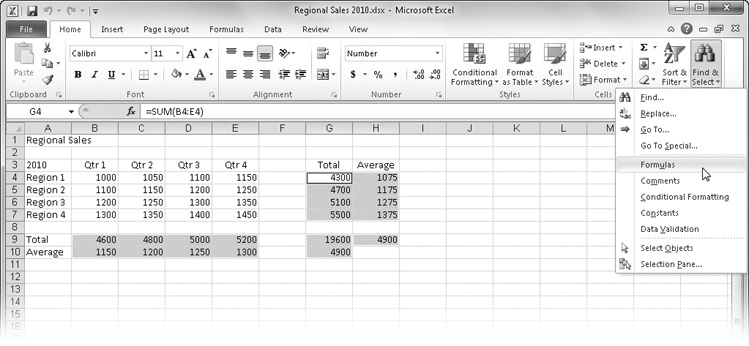
In Figure 6-5, we used the Formulas command to select all the formulas on the worksheet, which are highlighted by multiple selection rectangles. You can use these specialized selection commands for various purposes, such as applying specific formatting to formulas and constants or auditing worksheets for errant conditional formatting or data validation cells.
The two Go To commands are also helpful for finding and selecting a variety of worksheet elements. To quickly move to and select a cell or a range of cells, click Go To (or press F5) to open the Go To dialog box; then type a cell reference, range reference, or defined range name in the Reference box, and press Enter. You can also extend a selection using Go To. For example, to select A1:Z100, you can click A1, open the Go To dialog box, type Z100, and then press Shift+Enter.
Note
For more about selecting, see Finding and Replacing Stuff on page 240 and Selecting and Grouping Objects on page 421. For more information about defined range names and references, see Naming Cells and Cell Ranges on page 483 and Using Cell References in Formulas on page 468.
To move to another worksheet in the same workbook, open the Go To dialog box, and type the name of the worksheet, followed by an exclamation point and a cell name or reference.
For example, to go to cell D5 on a worksheet called Sheet2, type Sheet2!D5. To move to another worksheet in another open workbook, open the Go To dialog box, and type the name of the workbook in brackets, followed by the name of the worksheet, an exclamation point, and a cell name or reference. For example, to go to cell D5 on a worksheet called Sheet2 in an open workbook called Sales.xlsx, type [Sales.xlsx]Sheet2!D5.
Excel keeps track of the last four locations from which you used the Go To command and lists them in the Go To dialog box. You can use this list to move among these locations in your worksheet. This is handy when you’re working on a large worksheet or jumping around among multiple locations and worksheets in a workbook. Figure 6-6 shows the Go To dialog box displaying four previous locations.

When you click the Special button in the Go To dialog box (or the Go To Special command on the Find & Select menu), the dialog box shown on the right of Figure 6-6 opens, presenting additional selection options. You can think of the Go To Special dialog box as “Select Special” because you can use it to quickly find and select cells that meet certain specifications.
After you specify one of the Go To Special options and click OK, Excel highlights the cell or cells that match the criteria. With a few exceptions, if you select a range of cells before you open the Go To Special dialog box, Excel searches only within the selected range; if the current selection is a single cell or one or more graphic objects, Excel searches the entire active worksheet. The following are guidelines for using the Go To Special options:
Constants Refers to any cell containing static data, such as numbers or text, but not formulas.
Current Region Handy when you’re working in a large, complex worksheet and need to select blocks of cells. (Recall that a region is defined as a rectangular block of cells bounded by blank rows, blank columns, or worksheet borders.)
Current Array Selects all the cells in an array if the selected cell is part of an array range.
Last Cell Selects the cell in the lower-right corner of the range that encompasses all the cells that contain data, comments, or formats. When you select Last Cell, Excel finds the last cell in the active area of the worksheet, not the lower-right corner of the current selection.
Visible Cells Only Excludes from the current selection any cells in hidden rows or columns.
Objects Selects all graphic objects in your worksheet, regardless of the current selection.
Conditional Formats Selects only those cells that have conditional formatting applied. You can also click the Home tab and then click the Conditional Formatting command on the Find & Select menu.
Data Validation Using the All option, selects all cells to which data validation has been applied; Data Validation using the Same option selects only cells with the same validation settings as the currently selected cell. You can also click the Home tab and then click the Data Validation command on the Find & Select menu, which uses the All option.
Note
For more information about graphic objects, see Chapter 10. For more information about conditional formatting, see Formatting Conditionally on page 309.
Navigating Multiple Selections
Some of the Go To Special options—such as Formulas, Comments, Precedents, and Dependents—might cause Excel to select multiple nonadjacent ranges. But you might want to change the active cell without losing the multiselection. Or you might want to type entries into multiple ranges that you preselect so that you don’t have to reach for the mouse. Either way, you can move among cells within ranges, and between ranges, without losing the selection. For example, the worksheet shown here has three ranges selected:

To move the active cell through these ranges without losing the selection, press Enter to move down or to the right one cell at a time; press Shift+Enter to move up or to the left one cell at a time. Or press Tab to move to the right or down; press Shift+Tab to move to the left or up. So, in this worksheet, if you press Enter until cell A17 is selected, the next time you press Enter the selection jumps to the beginning of the next selected region, in this case cell A1. Subsequently pressing Enter selects A2, then B1, then B2, and so on, moving down and across until the end of the region (cell F2), and then to the next region (cell B4).
The Precedents and Dependents options in the Go To Special dialog box let you find all cells that are used by a formula or to find all cells upon which a formula depends. To use the Precedents and Dependents options, first select the cell whose precedents or dependents you want to find. When searching for precedents or dependents, Excel always searches the entire worksheet. When you select the Precedents or Dependents option, Excel activates the Direct Only and All Levels options:
Direct Only finds only those cells that directly refer to or that directly depend on the active cell.
All Levels locates direct precedents and dependents plus those cells indirectly related to the active cell.
Depending on the task, you might find the built-in auditing features of Excel to be just the trick. On the Formulas tab on the ribbon, the Formula Auditing group offers the Trace Precedents and Trace Dependents buttons. Rather than selecting all such cells, as the Go To Special command does, clicking these buttons draws arrows showing path and direction in relation to the selected cell.
Note
For more information, see Auditing and Documenting Worksheets on page 261.
The Row Differences and Column Differences options in the Go To Special dialog box compare the entries in a range of cells to spot potential inconsistencies. To use these debugging options, select the range before displaying the Go To Special dialog box. The position of the active cell in your selection determines which cells Excel uses to make its comparisons. When searching for row differences, Excel compares the cells in the selection with the cells in the same column as the active cell. When searching for column differences, Excel compares the cells in the selection with the cells in the same row as the active cell.
In addition to other variations, the Row Differences and Column Differences options look for differences in references and select those cells that don’t conform to the comparison cell. They also verify that all the cells in the selected range contain the same type of entries. For example, if the comparison cell contains a SUM function, Excel flags any cells that contain a function, formula, or value other than SUM. If the comparison cell contains a constant text or numeric value, Excel flags any cells in the selected range that don’t match the comparison value. The options, however, are not case-sensitive.