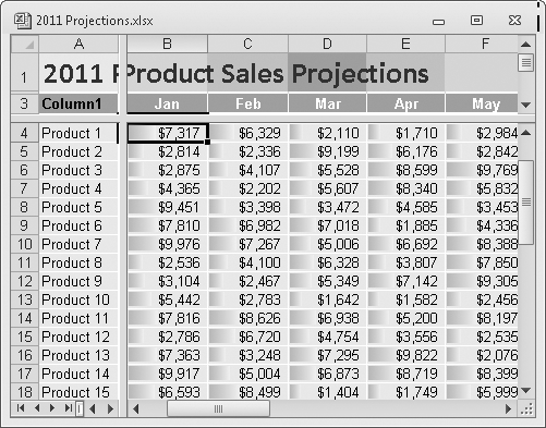
Worksheet panes let you view different areas of your worksheet simultaneously. You can split any worksheet in a workbook vertically, horizontally, or both vertically and horizontally and have synchronized scrolling capabilities in each pane. On the worksheet shown in Figure 6-17, columns B through M and rows 4 through 37 contain data. Column N and row 38 contain the totals. In Normal view, it’s impossible to see the totals and the headings at the same time.

Figure 6-17. You can scroll to display the totals in column N or row 38, but you won’t be able to see the headings.

It would be easier to navigate the worksheet in Figure 6-17 if it were split into panes. To do so, click the View tab on the ribbon, and click Split; the window divides into both vertical and horizontal panes simultaneously, as shown in Figure 6-18. You can use the mouse to drag either split bar to where you need it. If you double-click either split bar icon (located in the scroll bars, as shown in Figure 6-17), you divide the window approximately in half. When you rest your pointer on a split bar, it changes to a double-headed arrow.

Figure 6-18. With the window split, you can scroll each pane independently.

With the window split into four panes, as shown in Figure 6-18, four scroll bars are available (if not visible)—two for each direction. Now you can use the scroll bars to view columns B through N without losing sight of the product headings in column A. In addition, when you scroll vertically between rows 4 and 38, you always see the corresponding headings in row 3.

After a window is split, you can reposition the split bars by dragging. If you are ready to return your screen to its normal appearance, click the Split button again to remove all the split bars. You can also remove an individual split by double-clicking the split bar or by dragging the split bar to the top or right side of the window.

After you’ve split a window into panes, you can freeze the left panes, the top panes, or both panes by clicking the View tab on the ribbon, clicking Freeze Panes, and selecting the corresponding option, as shown in Figure 6-19. When you do so, you lock the data in the frozen panes into place. As you can see in Figure 6-19, the pane divider lines have changed from thick, three-dimensional lines to thin lines.

Figure 6-19. Freezing panes locks the top and/or left panes of a split window.

Notice also that in Figure 6-18, the sheet tabs are invisible because the horizontal scroll bar for the lower-left pane is so small. After freezing the panes, as shown in Figure 6-19, the scroll bar returns to normal, and the sheet tabs reappear.

After you freeze panes, scrolling within each pane works differently. You cannot scroll the upper-left panes in any direction. In the upper-right pane only the columns can be scrolled (right and left) and in the lower-left pane only the rows can be scrolled (up and down). You can scroll the lower-right pane in either direction.

Use the Zoom controls in the bottom-right corner of the screen (or click the View tab and use the Zoom button) to change the size of your worksheet display. Clicking the Zoom button displays a dialog box containing one enlargement option, three reduction options, and a Fit Selection option that determines the necessary reduction or enlargement needed to display the currently selected cells. Use the Custom box to specify any zoom percentage from 10 through 400 percent. The Zoom To Selection button enlarges or reduces the size of the worksheet to make all the selected cells visible on the screen. Clicking Zoom To Selection with a single cell selected zooms to the maximum 400 percent, centered on the selected cell (as much as possible) in an attempt to fill the screen with the selection.

For example, to view the entire worksheet shown in Figure 6-17, you can try different zoom percentages until you get the results you want. Better still, select the entire active area of the worksheet, and then click the Zoom To Selection button. Now the entire worksheet appears on the screen, as shown in Figure 6-20. Note that the zoom percentage resulting from clicking Zoom To Selection is displayed next to the Zoom control at the bottom of the screen.

Figure 6-20. Click the Zoom To Selection button with the active area selected to view it all on the screen.

Of course, reading the numbers might be a problem when your worksheet is zoomed “far out,” but you can select other reduction or enlargement sizes for that purpose. The Zoom option in effect when you save the worksheet is the displayed setting when you reopen the worksheet.

Suppose you want your worksheet to have particular display and print settings for one purpose, such as editing, but different display and print settings for another purpose, such as an on-screen presentation. By clicking the Custom Views button on the View tab, you can assign names to specific view settings, which include column widths, row heights, display options, window size, position on the screen, pane settings, the cells that are selected at the time the view is created, and, optionally, print and filter settings. You can then select your saved view settings whenever you need them rather than manually configuring the settings each time.

In the Custom Views dialog box, the Views list is empty until you click Add to save a custom view. All your custom views are saved with the workbook. Figure 6-21 shows the Custom Views dialog box with two views added, as well as the Add View dialog box you use to add them.

Figure 6-21. Click Add to name the current view and print settings in the Custom Views dialog box.