When you start a formula by typing an equal sign into a cell, you activate Enter mode. If you then click another cell, you don’t select it; instead, the cell’s reference is inserted in the formula. You can save time and increase accuracy when you enter cell references this way. For example, to enter references to cells A9 and A10 in a formula in cell B10, do the following:

When you click each cell, a marquee surrounds the cell, and Excel inserts a reference to the cell in cell B10. After you finish entering a formula, be sure to press Enter. If you do not press Enter but select another cell, Excel assumes you want to include that cell reference in the formula as well.

The active cell does not have to be visible in the current window for you to enter a value in that cell. You can scroll through the worksheet without changing the active cell and click cells in remote areas of your worksheet, in other worksheets, or in other workbooks as you build a formula. The formula bar displays the contents of the active cell no matter which area of the worksheet is currently visible.

Relative references—the type we’ve used so far in the sample formulas—refer to cells by their position in relation to the cell that contains the formula, such as “the cell two rows above this cell.” A relative reference to cell A1, for example, looks like this: =A1.

Absolute references refer to cells by their fixed position in the worksheet, such as “the cell located at the intersection of column A and row 2.” An absolute reference to cell A1 looks like this: =$A$1.

Mixed references contain a relative reference and an absolute reference, such as “the cell located in column A and two rows above this cell.” A mixed reference to cell A1 looks like this: =$A1 or =A$1.

Dollar signs in a cell reference indicate its “absoluteness.” If the dollar sign precedes only the letter (A, for example), the column coordinate is absolute, and the row is relative. If the dollar sign precedes only the number (1, for example), the column coordinate is relative, and the row is absolute.

Absolute and mixed references are important when you begin copying formulas from one location to another in your worksheet. When you copy and paste, relative references adjust automatically, but absolute references do not. For information about copying cell references, see How Copying Affects Cell References on page 472.

While you are entering or editing a formula, press F4 to change reference types quickly. The following steps show how:

When you use this technique to change reference types, click the formula bar to activate it, and then, before pressing F4, click in the cell reference you want to change or drag to select one or more cell references in the formula to change all the selected references at the same time.

You can refer to cells in other worksheets within the same workbook just as easily as you refer to cells in the same worksheet. For example, to enter a reference to cell A9 in Sheet2 into cell B10 in Sheet1, do this:

After you press Enter, Sheet1 once again becomes the active sheet. Select cell B10, and you can see that it contains the formula =Sheet2!A9.

The worksheet portion of the reference is separated from the cell portion by an exclamation point. Note also that the cell reference is relative, which is the default when you select cells to create references to other worksheets.

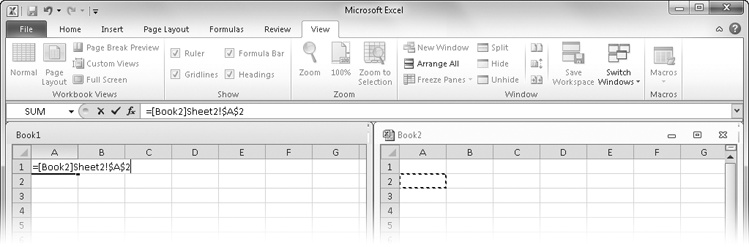
You can refer to cells in worksheets in separate workbooks in the same way you refer to cells in other worksheets within the same workbook. These references are called external references. For example, to enter a reference to Book2 in Book1, follow these steps:

Figure 12-1. Enter external references easily by clicking the cell to which you want to refer.

One of the handiest benefits of using references is the ability to copy and paste formulas. But you need to understand what happens to your references after you paste so that you can create formulas with references that operate the way you want them to operate.

Copying Relative References When you copy a cell containing a formula with relative cell references, Excel changes the references automatically relative to the position of the cell where you paste the formula. Referring to Figure 12-2, suppose you type the formula =AVERAGE(B4:E4) in cell F4. This formula averages the values in columns B through E.

Figure 12-2. Cell F4 contains relative references to the cells to its left.

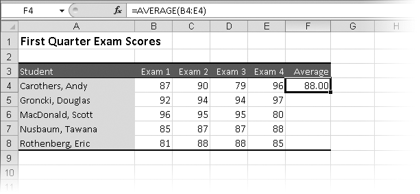
You want to include this calculation for the remaining rows as well. Instead of typing a new formula in each cell in column F, select cell F4 and press Ctrl+C to copy it (or click the Copy button in the Clipboard group on the Home tab). Then select cells F5:F8, click the arrow next to the Paste button on the Home tab, click Paste Special, and then select the Formulas And Number Formats option (to preserve the cell and border formatting). Figure 12-3 shows the results. Because the formula in cell F4 contains a relative reference, Excel adjusts the references in each copy of the formula. As a result, each copy of the formula calculates the average of the cells in the corresponding row. For example, cell F5 contains the formula =AVERAGE(B5:E5).

Figure 12-3. We copied the relative references from cell F4 to cells F5:F8.

Copying Absolute References If you want cell references to remain the same when you copy them, use absolute references. For example, in the worksheet on the left in Figure 12-4, cell B2 contains the hourly rate at which employees are to be paid, and cell C5 contains the relative reference formula =B2*B5. Suppose you copy the formula in C5 to the range C6:C8. The worksheet on the right in Figure 12-4 shows what happens: You get erroneous results. The formulas in cells C6:C8 should refer to cell B2, but they don’t. For example, cell C8 contains the incorrect formula =B5*B8.

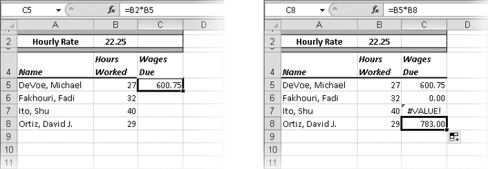
Figure 12-4. The formula in cell C5 contains relative references. We copied the relative formula in cell C5 to cells C6:C8, producing incorrect results.

Because the reference to cell B2 in the original formula is relative, it changes as you copy the formula to the other cells. To correctly apply the wage rate in cell B2 to all the calculations, you must change the reference to cell B2 to an absolute reference before you copy the formula.

To change the reference style, click the formula bar, click the reference to cell B2, and then press F4. The result is the following formula: =$B$2*B5.

When you copy this modified formula to cells C6:C8, Excel adjusts the second cell reference within each formula but not the first. In Figure 12-5, cell C8 now contains the correct formula: =$B$2*B8.

Figure 12-5. We created an absolute reference to cell B2 before copying the formula.

Copying Mixed References You can use mixed references in your formulas to anchor a portion of a cell reference. (In a mixed reference, one portion is absolute, and the other is relative.) When you copy a mixed reference, Excel anchors the absolute portion and adjusts the relative portion to reflect the location of the cell to which you copy the formula.

To create a mixed reference, you can press the F4 key to cycle through the four combinations of absolute and relative references—for example, from B2 to $B$2 to B$2 to $B2.

The loan payment table in Figure 12-6 uses mixed references (and an absolute reference). You need to enter only one formula in cell C6 and then copy it down and across to fill the table. Cell C6 contains the formula = –PMT($B6,$C$3,C$5) to calculate annual payments on a loan. We copied this formula to all the cells in the range C6:F10 to calculate payments using three additional loan amounts and four additional interest rates.

Figure 12-6. This loan payment table uses formulas that contain mixed references.

The first cell reference, $B6, indicates that we always want to refer to the values in column B but the row reference (Rate) can change. Similarly, the mixed reference, C$5, indicates we always want to refer to the values in row 5 but the column reference (Loan Amount) can change. For example, cell E8 contains the formula = –PMT($B8,$C$3,E$5). Without mixed references, we would have to edit the formulas manually in each of the cells in the range C6:F10.

So far, we have used the default worksheet and workbook names for the examples in this book. When you save a workbook, you must give it a permanent name. If you create a formula first and then save the workbook with a new name, Excel adjusts the formula accordingly. For example, if you save Book2 as Sales.xlsx, Excel changes the remote reference formula =[Book2]Sheet2!$A$2 to =[Sales.xlsx]Sheet2!$A$2. And if you rename Sheet2 of Sales.xlsx to February, Excel changes the reference to =[Sales.xlsx]February!$A$2. If the referenced workbook is closed, Excel displays the full path to the folder where the workbook is stored in the reference, as shown in the example =’C:Work[Sales.xlsx]February’!$A$2.

In the preceding example, note that apostrophes surround the workbook and worksheet portion of the reference. Excel adds the apostrophes around the path when you close the workbook. If you type a new reference to a closed workbook, however, you must add the apostrophes yourself. To avoid typing errors, it is best to work with the linked workbooks open and click cells to enter references so that Excel inserts them in the correct syntax for you.

The seemingly oxymoronic term numeric text refers to an entry that is not strictly numbers but includes both numbers and a few specific text characters. You can perform mathematical operations on numeric text values as long as the numeric string uses only the following characters in very specific ways:

0 1 2 3 4 5 6 7 8 9 . + - E e

In addition, you can use the / character in fractions. You can also use the following five number-formatting characters:

$ , % ( )

You must enclose numeric text strings in quotation marks. For example, if you type the formula =$1234+$123, Excel displays an error message. (The error message also offers to correct the error for you by removing the dollar signs.) But the formula =“$1234”+“$123” produces the result 1357 (ignoring the dollar signs). When Excel performs the addition, it automatically translates numeric text entries into numeric values.

The term text value refers to any entry that is neither a number nor a numeric text value (see the previous section); Excel treats the entry as text only. You can refer to and manipulate text values by using formulas. For example, if cell A1 contains the text First and you type the formula =A1 in cell A10, cell A10 displays First.

You can use the & (ampersand) operator to concatenate, or join, several text values. Extending the preceding example, if cell A2 contains the text Quarter and you type the formula =A1&A2 in cell A3, then cell A3 displays FirstQuarter. To include a space between the two strings, change the formula to =A1&” “&A2. This formula uses two concatenation operators and a literal string, or string constant (in this case, a space enclosed in quotation marks).

You can use the & operator to concatenate strings of numeric values as well. For example, if cell A3 contains the numeric value 867 and cell A4 contains the numeric value 5309, the formula =A3&A4 produces the string 8675309. This string is left-aligned in the cell because it’s considered a text value. (Remember, you can use numeric text values to perform any mathematical operation as long as the numeric string contains only the numeric characters listed in the previous section.)

Finally, you can use the & operator to concatenate a text value and a numeric value. For example, if cell A1 contains the text January and cell A3 contains the numeric value 2009, the formula =A1&A3 produces the string January2009.

INSIDE OUT Practical Concatenation

Depending on the kind of work you do, the text manipulation prowess of Excel may turn out to be the most important skill you learn in this book. If you deal with a lot of mailing lists, for example, you probably use a word-processing application such as Microsoft Word. But you might find that Excel has the tools you’ve been wishing for, and it just might become your text manipulation application of choice.

Suppose you have a database of names in which the first and last names are stored in separate columns. This example shows you how to generate lists of full names:

We created the full names listed in columns D and E using formulas like the one visible in the formula bar. For example, the formula in cell D2 is =B2&” “&A2, which concatenates and reverses the contents of the cells in columns A and B and adds a space character in between. The formula in cell E2 (=A2&”, “&B2) reverses the position of the first and last names and adds a comma before the space character. For another nifty—and related—trick, see the sidebar Practical Text Manipulation on page 548.