
The options used most often to affect the appearance of your printed pages are available on the Page Layout tab on the ribbon, shown in Figure 11-1. This is the central control panel for setting up paper sizes, margins, and page orientation, as well as for working with page breaks, print areas, and other printing options. For even more control over page layout, click the dialog box launcher in the Page Setup group on the Page Layout tab to display the Page Setup dialog box, also shown in Figure 11-1.
The new File tab in Excel 2010, aka Backstage view, now includes the most-often-used options as well and provides some visual feedback about what all these things actually do. Plus, a print preview is displayed on the right side of the screen and dynamically displays the settings you choose from the options on the left side. Click the File tab, and then click Print to display a screen similar to the one shown in Figure 11-2.
The settings you use most frequently are duplicated in several places. Most of what you need is on the Page Layout tab of the ribbon, in the Print category on the File tab, and, of course, in the Page Setup dialog box. These settings control page orientation, scaling, paper size, print quality, and page numbering.
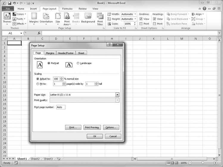
Figure 11-1. The Page Layout tab on the ribbon and the Page Setup dialog box control most printing options.

The Orientation button on the Page Layout tab offers two options: Portrait and Landscape. These options determine whether Excel prints your worksheet vertically (Portrait) or horizontally (Landscape). Portrait, the default setting, offers more room for rows but less room for columns. Select Landscape if you have more columns but fewer rows on each page. You can also find these options on the Page tab in the Page Setup dialog box and in the Print category on the File tab.
The Size button on the Page Layout tab includes options for nearly every size of paper available (not just the sizes supported by your printer). You can additionally control the quality of your printout by clicking the Size button and then clicking More Paper Sizes (or clicking the dialog box launcher in the Page Setup group) to display the Page tab in the Page Setup dialog box. The same options are duplicated in the Print category on the File tab.

Figure 11-2. Click the File tab, and then click Print to display the most popular printing options, as well as Print Preview, in Backstage view.
On the Page tab of the Page Setup dialog box, the Print Quality drop-down list shows the quality options available for your printer. A laser printer, for example, might offer print-quality settings of 600 dots per inch (dpi), 300 dpi, and 150 dpi. Higher dpi settings look better, but a page takes longer to print. If the Print Quality drop-down list is not available, you might be able to adjust these settings—and more—using your printer driver’s dialog box, which you can access by clicking the Options button on the Page tab in the Page Setup dialog box. You can also access the printer driver dialog box by clicking Printer Properties in the Print category on the File tab.
Note
For more information about printer drivers, see Setting Printer Driver Options on page 456.
There are several ways to specify a reduction or enlargement ratio for your printouts. Using the Scale To Fit group on the Page Layout tab, you can override the default size of your printouts in one of two ways: by specifying a scaling factor (from 10 percent through 400 percent) or by fitting the printout to a specified number of pages. Excel always scales in both the horizontal and vertical dimensions.
The Width and Height controls on the Page Layout tab, shown in Figure 11-1, normally display Automatic, which means the worksheet prints at full size on as many pages as necessary. In these drop-down lists, choose a number of pages to constrain the printout. For example, choosing 2 Pages in the Width list (and leaving Height set to Automatic) scales the print area of the worksheet so that it spans two pages at its widest point, filling as many pages in length as necessary. Choosing 2 Pages in the Height list (and leaving Width set to Automatic) scales the print area of the worksheet so that it is only two pages long, filling as many pages in width as necessary.
The Fit To options in the Page Setup dialog box give you more precise control over scaling. These mirror the Height and Width controls on the Page Layout tab. To return to a full-size printout, select the Adjust To option and type 100 in the % Normal Size box.
You can also use the Scaling options in the File tab’s Print category. The Print category, shown in Figure 11-3, allows you to specify scaling and other options on the fly just before you send the worksheet to the printer.
If you want to control the numbering of pages in your printout’s header or footer—an essential tool when printing multipage worksheets—use the First Page Number box on the Page tab in the Page Setup dialog box. You can type any starting number, including 0 or negative numbers. By default, this option is set to Auto.

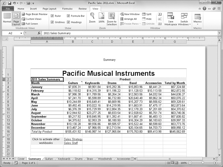
Page Layout view represents a major upgrade to the worksheet-printing workflow in comparison with the “old” ways of doing things. Not only can you see the page as it will print, as you can with Print Preview, but Excel is fully functional in Page Layout view, so you can make changes and see the results immediately. Click the Page Layout button on the View tab, shown in Figure 11-4. This might become your preferred working environment, if you don’t mind the slight slowdown in performance that comes with a more graphically intensive interface.
In Page Layout view, you can do the following:
Drag the edge between the shaded and white areas on the rulers to adjust margins.
Drag lines between row and column headers to adjust row height and column width.
Refer to the rulers to see the actual dimensions of your data relative to the printed page.
Click the Page Layout tab and change settings in the Page Setup group to see the changes immediately reflected on your screen.
Click other tabs on the ribbon to zoom, apply formatting, and add formulas, graphics, charts, and so on. Note, however, that Page Layout view can be set separately on each sheet, so switching to another sheet might also switch you back to Normal view.
In fact, we couldn’t find anything you can’t do in Page Layout view. Page Layout view is applied per worksheet; you can specify a different view for each open worksheet, and the settings are saved with the workbook.
Note
You can also use the three tiny buttons at the bottom of the screen next to the Zoom slider to change the view. The first button activates Normal view, the second activates Page Layout view, and the third activates Page Break Preview. For more about Page Break Preview, see Adjusting Page Breaks on page 457.
You can adjust the margins of your printouts to allow the maximum amount of data to fit on a page, to customize the amount of space available for headers and footers, or to accommodate special requirements such as three-hole-punched paper, company logos, and so on. The Margins button on the Page Layout tab, shown in Figure 11-5, provides three settings that should meet most of your needs: Normal, Wide, and Narrow. These settings refer to the size of the margins, not the size of the printed area. For example, to fit more data on a page, use the Narrow setting. Note that when you apply your own margin settings, the Last Custom Setting command appears as the first item on the Margins menu, as Figure 11-5 shows. This command does not appear unless you specify your own margin settings. These commands also appear in the Print category on the File tab.

The Margins tab in the Page Setup dialog box offers precise control over the top, bottom, left, and right margins of your printed worksheets. You can display the Margins tab, shown in Figure 11-6, by clicking the Margins button and then clicking Custom Margins.
When you click in any of the text boxes on the Margins tab, the corresponding margin line is highlighted in the sample page in the middle of the dialog box, showing you where the selected margin will appear.
If you want a header or footer to appear on each page, the top and bottom margins need to be large enough to accommodate them. For more information about setting up a header and footer, see Creating a Header and Footer below.


The easiest way to create headers and footers is to click the Header & Footer button on the Insert tab, which simultaneously displays the Header & Footer Tools Design tab, switches the worksheet to Page Layout view, and activates the header for editing, as shown in Figure 11-7.

Figure 11-7. Click the Header & Footer button on the Insert tab to display the Header & Footer Tools Design tab.
Both the Header and Footer areas in Page Layout view consist of edit boxes in three sections—left, center, and right—that are formatted with the corresponding justification (that is, the contents of the box on the right are right-justified). Use these edit boxes to insert and format headers and footers using buttons on the Header & Footer Tools Design tab:
Header & Footer group These buttons display menus of predesigned headers and footers, shown as they appear when printed. For example, if you click Page 1 Of ? on the Header menu, the proper code is inserted in the header. If you then click the inserted information in the header, you can see the underlying code—much like a formula in a cell—that produces the result: Page &[Page] of &[Pages]. You don’t really need to know these codes; buttons are available to create them for you.
Page Number Inserts the page number in the selected section.
Number Of Pages Inserts the total number of pages in the selected section; typically used in conjunction with the page number in a “Page X of Y” construction.
Current Date Inserts the date of printing.
Current Time Inserts the time of printing.
File Path Inserts the folder path and file name of the workbook.
File Name Inserts only the file name of the current workbook.
Sheet Name Inserts the name of the current worksheet.
Picture Displays the Insert Picture dialog box. (See Adding Pictures to Headers and Footers on page 449.)
Format Picture Displays the Format Picture dialog box, letting you adjust the settings of an inserted picture.
Navigation group The Go To Header and Go To Footer buttons are simply quick ways to jump between the corresponding edit boxes at the top and bottom of the page.
Different First Page Specifies a different header and footer for the first page only.
Different Odd & Even Pages Specifies different headers and footers for even and odd pages; typically used to create balanced two-page spreads when you print a worksheet double-sided.
Scale With Document Selected by default; clear this check box if you want headers and footers to remain unchanged even if you enlarge or shrink the rest of the document.
Align With Page Margins Selected by default; clear this check box if you want the headers and footers to remain fixed, unaffected by changes to the margins.
Note
By default, Excel prints footers .3 inch from the bottom edge and headers .3 inch from the top edge, but you can change this on the Margins tab in the Page Setup dialog box.
Excel uses codes to represent dynamic data in your headers and footers, such as the current time represented by &[Time]. Fortunately, you don’t have to learn these codes to create headers and footers. Click the edit box where you want the information to appear, and then click the appropriate buttons to add the information to your header or footer. Here are some things to remember about editing headers and footers:
To include text in a header or footer, just click a text box and start typing. You need to add spaces between text and inserted code elements, as well as between adjacent code elements.
An ampersand (&) always precedes a code element, so never insert anything between the ampersand and its code. To include an actual ampersand in your header or footer, type two ampersands.
To apply formatting, use the small, ghostly toolbar that appears when you select text in an edit box. Or, because the worksheet is in Page Layout view, you can click the Home tab and use the formatting tools in the Font group as well as the editing tools in the Clipboard group.
As in cells, if you enter more information in any of the header or footer edit boxes than can be displayed, the information spills over into adjacent edit boxes. Yes, you can enter too much data, actually causing text to overlap, but you’ll see it immediately because you are working in Page Layout view.
To remove header or footer information, click the None option at the top of the Header or Footer button menu, or simply delete the contents of the corresponding edit boxes in Page Layout view.
The Page Setup dialog box contains the old-school interface for Excel’s header and footer features. You can still use it, but it affords little advantage over the Header & Footer Tools Design tab. Click the Page Layout tab, click the dialog box launcher in the Page Setup group to display the Page Setup dialog box, and then click the Header/Footer tab, as shown in Figure 11-8.
The drop-down lists that appear immediately under the words Header and Footer offer the same lists of predefined options as the eponymous buttons on the Header & Footer Tools Design tab. And the check box options in the dialog box mirror the ones in the Options group on the tab. The three buttons at the bottom of the dialog box are really the only things that offer a little added value here. The Print button takes you directly to the Print screen in Backstage view, and the Print Preview button actually takes you to the same place, since Print Preview now appears in Backstage view as well. The Options button takes you directly to your printer’s Properties dialog box. Click the Custom Header button to display a dialog box similar to the one shown in Figure 11-9.
The Header (and identical Footer) dialog box does almost all the things that the Header & Footer Tools Design tab does. The only difference here is the addition of the Format Text button (the first button on the left), which displays the Font dialog box shown in Figure 11-9.


You can add pictures to custom headers and footers by using the Picture and Format Picture buttons (refer to Figure 11-7). For example, you can insert pictures to add company logos or banners to your documents. Click the Picture button to access the Insert Picture dialog box (a version of the standard Open dialog box), which you use to locate the picture you want to insert. When you insert the picture, Excel includes the code &[Picture], and the image is displayed in the edit box. (Unlike with other header and footer codes, you can’t just type this code—you have to use the Picture button.)
After you insert a picture, click the Format Picture button to specify the size, brightness, and contrast of the picture and to rotate, scale, or crop the picture. (You can’t directly manipulate header or footer pictures—you must use the Format Picture button.) It might take some trial and error to obtain the result you want, adjusting the size of the picture as well as the top or bottom margins to accommodate it. Figure 11-10 shows a sample of a picture used in a header, with the worksheet displayed in Page Layout view.
To arrive at the example shown in Figure 11-10, we did the following:
In the left section, we added the date and changed the font to 10-point, italic Arial Black.
In the center section, we inserted a picture; then we clicked Format Picture and reduced its size.
In the right section, we added the time and changed the font to 10-point, italic Arial Black.
We clicked the Page Layout tab and clicked the dialog box launcher button in the Page Setup group to display the Page Setup dialog box.
We selected both the Vertically and Horizontally check boxes below Center On Page on the Margins tab in the Page Setup dialog box.
We dragged the top margin down using the side ruler in Page Layout view enough to accommodate the graphic.

Clicking the dialog box launcher in the Page Setup group on the Page Layout tab displays the Page Setup dialog box. Click the Sheet tab, shown in Figure 11-11, to access settings specific to the active worksheet. You can specify different worksheet options for each worksheet in a workbook. (You can also display the Sheet tab by clicking the Print Titles button on the Page Layout tab.)

Figure 11-11. The Sheet tab in the Page Setup dialog box stores the print area and print titles data.
If you do not specify an area to print, Excel prints the entire active area of the selected worksheet(s). If you don’t want to print the entire worksheet, you can specify an area to print by using the Print Area button on the Page Layout tab. First, select the range or ranges you want to print, click Print Area on the Page Layout tab, and then click Set Print Area. To clear this setting, click the Print Area button and click Clear Print Area. You can specify a print area setting for each worksheet, and the settings are saved with the workbook.
The print area settings are stored in the first box on the Sheet tab in the Page Setup dialog box, which you can also use to set or edit the print area. To do so, click the Print Titles button on the Page Layout tab (a quick way to display the Page Setup dialog box). Click in the Print Area box, and then drag to select the cells on the worksheet you want to include. When you do this, the dialog box collapses so you can see more of the worksheet, and Excel inserts the cell range reference of the area you select in the Print Area box, as shown in Figure 11-11. You can select multiple nonadjacent cell ranges by selecting a range, typing a comma, and then selecting the next range. Each range you select prints on a separate page.
Note
To remove a print area definition, you can return to the Page Setup dialog box and delete the cell references. You can also use the Define Name dialog box by pressing Ctrl+F3 and deleting the name Print_Area. For more information, see Naming Cells and Cell Ranges on page 483.
On most worksheets, the column and row labels that identify your data appear in only the first couple of columns and top few rows. When Excel breaks up a large report into pages, those important column and row labels might appear only on the first page of the printout. You use the Print Titles feature to force Excel to print the contents of one or more columns, one or more rows, or a combination of columns and rows on every page of a report.
Suppose you want to print the contents of column A and rows 1, 2, and 3 on all the pages of the report shown in Figure 11-11:
Click the Print Titles button on the Page Layout tab to display the Page Setup dialog box, open to the Sheet tab.
Click in the Rows To Repeat At Top text box, and then select the headings for the first three rows. (To select multiple contiguous row headings, drag through them.)
Click in the Columns To Repeat At Left text box, and then select the column A heading (or any cell in column A).
Figure 11-12 shows the result in Page Layout view. Notice that the column containing the product numbers appears on both pages displayed in Page Layout view. If you did not use print titles, the first column on the second page of the printout would display the June totals column instead of the product numbers. You can specify separate print titles for each worksheet in your workbook. Excel remembers the titles for each worksheet.

Note
To remove your print title definitions, you can return to the Page Setup dialog box and delete the cell references. You can also use the Define Name dialog box by pressing Ctrl+F3 and deleting the name Print_Titles. For more information, see Naming Cells and Cell Ranges on page 483.
By default, Excel does not print gridlines or row and column headings, regardless of whether they are displayed on your worksheet. If you want to print gridlines or headings, select the corresponding Print check box in the Sheet Options group on the Page Layout tab. You can also select the Gridlines or Row And Column Headings check box on the Sheet tab in the Page Setup dialog box.
Comments are annotations you create by clicking New Comment on the Review tab on the ribbon. To be sure the comments in your worksheet are included with your printout, select one of the Comments options on the Sheet tab in the Page Setup dialog box. If you select At End Of Sheet from the drop-down list, Excel adds a page to the end of the printout and prints all your notes together, starting on that page. If you select As Displayed On Sheet, Excel prints the comments as pop-up windows wherever they are located on a worksheet. The latter option might cause the comments to obscure worksheet data.
Note
You can display all comments on the worksheet by clicking the Show All Comments button on the Review tab on the ribbon. This gives you an idea of how the worksheet will look when printed if you select the As Displayed On Sheet option in the Page Setup dialog box.
The drop-down list cryptically labeled Cell Errors As on the Sheet tab in the Page Setup dialog box gives you options for how error codes displayed on the worksheet should be printed. Ordinarily, error codes such as #NAME? are printed just as they appear on your screen, but you can change this so that cells containing error codes print as blank cells or with a double hyphen (--) or #NA displayed instead of the error code.
Note
For more about creating comments, see Adding Comments to Cells on page 272. For more about error codes, see Understanding Error Values on page 479.
If your printer offers a draft-quality mode, you can obtain a quicker, though less attractive, printout by selecting the Draft Quality check box on the Sheet tab in the Page Setup dialog box. This option has no effect if your printer has no draft-quality mode and is most useful for dot matrix or other slow printers.
If you’ve assigned colors and patterns to your worksheet, but you want to see what it will look like when it’s printed on a black-and-white printer, select the Black And White check box on the Sheet tab in the Page Setup dialog box, which tells Excel to use only black and white when printing and previewing. You can see the results by clicking the Print Preview button in the Page Setup dialog box, which is just a handy way of getting to the Print screen in Backstage view—the same place you go by clicking the File tab on the ribbon and clicking Print.
When you print a large report, Excel breaks the report into page-size sections based on the current margin and page-size settings. If the print range is both too wide and too deep to fit on a single page, Excel ordinarily works in “down and then over” order. For example, suppose your print range measures 120 rows by 20 columns and that Excel can fit 40 rows and 10 columns on a page. Excel prints the first 40 rows and first 10 columns on page 1, the second 40 rows and first 10 columns on page 2, and so on, until it prints all the rows and starts at the top of the next 10 columns. If you prefer to have Excel print each horizontal chunk before moving to the next vertical chunk, select the Over, Then Down option on the Sheet tab in the Page Setup dialog box.