
When you copy an item, Excel 2010 saves it in memory, using a temporary storage area called the Clipboard. You capture the contents as well as the formatting and any attached comments or objects.
Note
For more information about comments, see Auditing and Documenting Worksheets on page 261. For more information about objects, see Chapter 10.
When you copy or cut cells, a marquee appears around the cell. (We used to refer to this scrolling dotted line as marching ants.) This marquee indicates the area copied or cut. After you paste, the marquee disappears when you’re cutting, but it persists when you’re copying so that you can keep pasting.

The Cut and Copy buttons on the Home tab are useful, but you should know the keyboard shortcuts for the quintessential editing commands listed in Table 8-1. You can click the equivalent buttons on the ribbon, but really, if you never learn another keyboard shortcut, learn these.
After you copy, you can paste more than once. As long as the marquee is visible, you can continue to paste the information from the copied cells. You can copy this information to other worksheets or workbooks without losing your copy area marquee. The marquee persists until you press Esc or perform any other editing action. The area you select for copying must be a single rectangular block of cells. If you try to copy nonadjacent ranges, you get an error message.
Although you cannot copy nonadjacent selections, you can use the Collect And Copy feature to copy (or cut) up to 24 separate items and then paste them where you want them—one at a time or all at once. You do this by displaying the Clipboard task pane shown in Figure 8-1 by clicking the dialog box launcher next to the word Clipboard on the Home tab on the ribbon.
Ordinarily when copying, you can work with only one item at a time. If you copy several items in a row, only the last item you copy is stored on the Clipboard. However, if you first display the Clipboard task pane and then copy or cut several items in succession, each item is stored in the task pane, as shown in Figure 8-1.
You can change the regular collect-and-copy behavior so that Excel collects items every time you copy or cut regardless of whether the Clipboard task pane is present. To do so, click the Options button at the bottom of the Clipboard task pane (see Figure 8-1), and click Collect Without Showing Office Clipboard or Show Office Clipboard Automatically, depending on whether you want the task pane to appear. The latter option activates an additional option, Show Office Clipboard When Ctrl+C Pressed Twice, which is one of the “automatic” methods.
Previewing Before You Paste
New in Excel 2010 is the paste preview feature, which allows you to see what a particular paste option looks like before you commit to actually pasting. After you copy or cut a cell or range, select the destination cell where you want to paste. Click the Paste menu on the Home tab (or right-click and use the Paste Options buttons on the shortcut menu). When you hover the mouse over each button, the result of that option is displayed on the worksheet in the specified location. In the following figure, we copied cells A1:A4, right-clicked cell C2 to display the shortcut menu, and then hovered over the Paste Options buttons:

The Paste menu on the Home tab is usually enough out of the way that it won’t obscure the area of the sheet that you’re working on. And since the shortcut menu appears where you right-click, you would think that it would always be in the way. But as you can see in the figure, it “ghosts” itself when you use the paste preview feature. For more about paste options in general, see Pasting Selectively Using Paste Special on page 203, and for information about the Transpose command in particular, see Transposing Entries on page 208.
Each time you copy or cut an item, a short representation of the item appears in the Clipboard task pane. Figure 8-1 shows four items in the Clipboard task pane. You can paste any or all of the items wherever you choose. To paste a single item from the Clipboard task pane, first select the location where you want the item to go, and then click the item in the task pane. To empty the Clipboard task pane for a new collection, click the Clear All button.

After you copy, press Ctrl+V to paste whatever you copied. It’s a no-brainer. However, did you know that if you select a range of cells before pasting, Excel fills every cell in that range when you paste? Figure 8-2 illustrates this.

Figure 8-2. Before you paste, select more cells than you copied to create multiple copies of your information.
In Figure 8-2, we did the following:
Copied cell A1 and then selected the range C1:C12 and pasted, resulting in Excel repeating the copied cell in each cell in the selected range.
Copied Cells A1:A4 and then selected the range E1:E12 and pasted, resulting in Excel repeating the copied range within the range.
Copied cells A1:A4 and then selected cell G1 and pasted, resulting in an exact duplicate of the copied range.
Copied cells A1:A4 and then selected the range A15:G15 and pasted, resulting in Excel repeating the copied range in each selected column.
Notice in Figure 8-2 that we clicked the floating Paste Options button that appears near the lower-left corner of the pasted range. This button appears whenever and wherever you paste, offering actions applicable after pasting—a sort of “Smart Paste Special.” (Similar floating buttons offering context-triggered options appear after performing actions other than pasting, too.) The best part is that you can try each action in turn. Keep selecting paste options until you like what you see, and then press Enter. The following describes the most interesting items on the Paste Options menu:
Formulas Pastes all cell contents, including formulas, but no formatting.
Formulas And Number Formatting Pastes all cell contents, including formulas and number formats, but no text formats.
No Borders Pastes everything but borders.
Transpose Flips a column of data into a row and vice versa.
Values Pastes cell contents and the visible results of formulas (not the formulas themselves) without formatting.
Values And Number Formatting Pastes cell contents and the visible results of formulas (not the formulas themselves); retains number formats, but not text formats.
Values And Source Formatting Pastes cell contents and the visible results of formulas (not the formulas themselves), plus all the copied or cut formats.
Keep Source Column Widths Retains column widths. This option is like normal pasting with the added action of “pasting” the column width.
Formatting Leaves the contents of the destination cells alone and transfers the formatting. This works in the same way as the Format Painter button, located in the Clipboard group on the Home tab.
Paste Link Instead of pasting the contents of the cut or copied cells, pastes a reference to the source cells, ignoring the source formatting.
Picture Pastes an image of the selected cells as a static graphic object.
Linked Picture Pastes an image of the selected cells as a dynamic graphic object. If you make any changes to the original cells, the changes are reflected in the graphic object. This is handy for monitoring remote cells.
When you cut rather than copy cells, subsequent pasting places one copy in the selected destination, removes the copied cells from the Clipboard, removes the copied data from its original location, and removes the marquee. When you perform a cut-and-paste operation, the following rules apply:
Excel clears both the contents and the formats from the cut range and transfers them to the cells in the paste range. Excel adjusts any formulas outside the cut area that refer to the cells that were moved.
The area you select for cutting must be a single rectangular block of cells. If you try to select nonadjacent ranges, you get an error message.
Regardless of the size of the range you select before pasting, Excel pastes only the exact size and shape of the cut area. The upper-left corner of the selected paste area becomes the upper-left corner of the moved cells.
Excel overwrites the contents and formats of any existing cells in the range where you paste. If you don’t want to lose existing cell entries, be sure your worksheet has enough blank cells below and to the right of the cell you select as the upper-left corner of the paste area to hold the entire cut area.
You cannot use Paste Special after cutting. Furthermore, no “floating button” menus appear when you paste after cutting.
Paste Special is quite possibly the most useful (and most used) power-editing feature. You can use this feature in many ways, but probably the most popular is copying the value in a cell without copying the formatting or the underlying formula. After you copy a cell or cells, click the Paste menu on the Home tab, and click Paste Special to display the Paste Special dialog box, shown in Figure 8-3. (You must copy to use Paste Special. When you cut, Paste Special is unavailable.) The most popular Paste Special actions are directly accessible as commands on the Paste menu on the Home tab, as shown on the left in Figure 8-3.
Note
The Paste menu is actually a button with a downward-pointing arrow below it; clicking the button is equivalent to clicking the Paste command. To display the menu shown on the left in Figure 8-3, click the arrow.
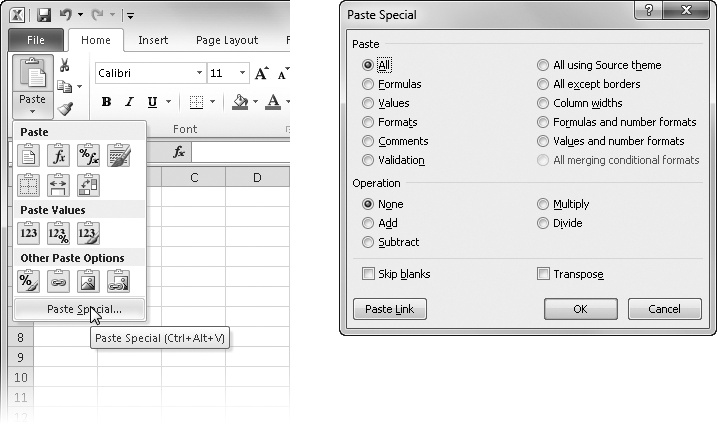
Figure 8-3. Paste Special is probably the most popular power-editing feature, and its most often used options are available as commands on the Paste menu.
Note
You can also open the Paste Special dialog box by right-clicking the cell where you want to paste and then clicking Paste Special.
Here’s what the Paste Special options do:
All Predictably, pastes all aspects of the selected cell, which is the same as clicking the Paste command.
Formulas Transfers only the formulas from the cells in the copy range to the cells in the paste range, adjusting relative references. This option is also available as a command on the Paste menu.
Values Pastes static text, numeric values, or only the displayed values resulting from formulas. This option is also available as the Paste Values command on the Paste menu.
Formats Transfers only the formats in the copy range to the paste range.
Comments Transfers only comments attached to selected cells.
Validation Pastes only the data validation settings you have applied to the selected cells.
All Using Source Theme Transfers the copied data and applies the theme from the copied cells.
All Except Borders Transfers data without disturbing the border formats you spent so much time applying. This option is also available as the No Borders command on the Paste menu.
Column Widths Transfers only column widths, which is handy when trying to make a worksheet look consistent for presentation.
Formulas And Number Formats Transfers only formulas and number formats, which is helpful when you are copying formulas to previously formatted areas. Usually, you want the same number formats applied to formulas you copy, wherever they happen to go.
Values And Number Formats Transfers only the resulting values (but not the formulas) and number formats.
All Merging Conditional Formats Transfers cell contents and formats, and merges any conditional formats in the copied cells with those found in the destination range. Copied conditions take precedence if there is a conflict.

Note
For more information about themes, see Using Themes and Cell Styles on page 300. For more about conditional formatting, see Formatting Conditionally on page 309.
Because the All option pastes the formulas, values, formats, and cell comments from the copy range into the paste range, it has the same effect as clicking Paste, probably making you wonder why Excel offers this option in the Paste Special dialog box. That brings us to our next topic—the Operation options.
You use the options in the Operation area of the Paste Special dialog box to mathematically combine the contents of the copied cells with the contents of the cells in the paste area. When you select any option other than None, Excel does not overwrite the destination cell or range with the copied data. Instead, it uses the specified operator to combine the copy and paste ranges.
For example, say you want to get a quick list of combined monthly totals for the Northern and Eastern regions in Figure 8-4. First, copy the Northern Region figures to an empty area of the worksheet, and then copy the Eastern Region numbers; select the first cell in the column of values that you just copied and click Paste Special. You then select the Values and Add options in the Paste Special dialog box, and after clicking OK, you get the result shown at the bottom of Figure 8-4.

Figure 8-4. We used the Values option in the Paste Special dialog box to add the totals from the Eastern Region to those of the Northern Region.
The other options in the Operation area of the Paste Special dialog box combine the contents of the copy and paste ranges using the appropriate operators. Just remember that the Subtract option subtracts the copy range from the paste range, and the Divide option divides the contents of the paste range by the contents of the copy range. Also note that if the copy range contains text entries and you use Paste Special with an Operation option (other than None), nothing happens.
Select the Values option when you use any Operation option. As long as the entries in the copy range are numbers, you can use All, but if the copy range contains formulas, you’ll get “interesting” results. As a rule, avoid using the Operation options if the paste range contains formulas.
The Paste Link button in the Paste Special dialog box, shown in Figure 8-4, is a handy way to create references to cells or ranges. Although the Paste Special dialog box offers more options, using the Paste Link command on the Paste menu on the Home tab is more convenient. When you click Paste Link, Excel enters an absolute reference to the copied cell in the new location. For example, if you copy cell A3, then select cell B5, click the Paste menu, and then click Paste Link, Excel enters the formula =$A$3 in cell B5.
If you copy a range of cells, Paste Link enters a similar formula for each cell in the copied range to the same-sized range in the new location.
Note
For more information about absolute references, see Understanding Relative, Absolute, and Mixed References on page 469.
The Paste Special dialog box contains a Skip Blanks check box that you can select when you want Excel to ignore any blank cells in the copy range. If your copy range contains blank cells, Excel usually pastes them over the corresponding cells in the paste area. As a result, empty cells in the copy range overwrite the contents, formats, and comments in corresponding cells of the paste area. When you select Skip Blanks, however, the corresponding cells in the paste area are unaffected by the copied blanks.
One of the often-overlooked but extremely useful Paste Special features is Transpose, which helps you reorient the contents of the copied range when you paste—that is, data in rows is pasted into columns, and data in columns is pasted into rows. (This option is also available as a command on the Paste menu.) For example, in Figure 8-5, we copied the data shown in cells B3:E3, and then we selected cell J3 and clicked Transpose on the Paste menu on the Home tab. This works both ways. If we subsequently select the range just pasted and click Transpose again, the data is pasted in its original orientation.

Figure 8-5. We copied cells B3:E3, selected cell J3, and then clicked Home, Paste, Transpose to redistribute the row of labels into a column of labels.
Tip
INSIDE OUT Using Paste Values with Arrays
As with any other formula, you can convert the results of an array formula to a series of constant values by copying the entire array range and—without changing your selection—clicking the Home tab, Paste, Paste Values. When you do so, Excel overwrites the array formulas with their resulting constant values. Because the range now contains constant values rather than formulas, Excel no longer treats the selection as an array. For more information about arrays, see Using Arrays on page 512.
Note
If you transpose cells containing formulas, Excel transposes the formulas and adjusts cell references. If you want the transposed formulas to continue to correctly refer to nontransposed cells, be sure that the references in the formulas are absolute before you copy them. For more information about absolute cell references, see Using Cell References in Formulas on page 468.
The Hyperlink command on the Insert tab has a specific purpose: to paste a hyperlink that refers to the copied data in the location you specify. When you create a hyperlink, it’s as though Excel draws an invisible box, which acts like a button when you click it, and places it over the selected cell.
Hyperlinks in Excel are similar to Web links that, when clicked, launch a Web page. You can add hyperlinks in your workbooks to locations on the Web—a handy way to make related information readily available. You can use hyperlinks to perform similar tasks among your Excel worksheets, such as to provide an easy way to access other worksheets or workbooks that contain additional information. You can even create hyperlinks to other Microsoft Office documents, such as a report created in Microsoft Word or a Microsoft PowerPoint presentation.
Within Excel, you create a hyperlink by copying a named cell or range, navigating to the location where you want the hyperlink (on the same worksheet, on a different worksheet, or in a different workbook), and then clicking Insert, Hyperlink. To create a hyperlink in and among Excel worksheets and workbooks, you must first assign a name to the range to which you want to hyperlink. (The easiest method is to select the cell or range and type a name in the Name box at the left end of the formula bar.) Note that hyperlinks differ from Excel links, which are actually formulas.
Note
For more information, see Pasting Links on page 207. For information about defining names, see Naming Cells and Cell Ranges on page 483. For more information about hyperlinks, see Chapter 26.
When you rest your pointer on a hyperlink, a ScreenTip appears showing you the name and location of the document to which the hyperlink is connected, as shown in Figure 8-6.

To use a hyperlink, just click it. To select the cell containing the hyperlink without activating the link, hold the mouse button down until the pointer changes to a cross, and then release the mouse button. To edit or delete a hyperlink, right-click it, and then click Edit Hyperlink or Remove Hyperlink.
Sometimes referred to as direct cell manipulation, this feature lets you quickly drag a cell or range to a new location. It’s that simple. When you select a cell or range, move the pointer over the edge of the selection until the four-headed arrow pointer appears, and then click the border and drag the selection to wherever you like. As you drag, an outline of the selected range appears, which you can use to help position the range correctly.
To copy a selection rather than move it, hold down the Ctrl key while dragging. The pointer then appears with a small plus sign next to it, as shown in Figure 8-7, which indicates you are copying rather than moving the selection.
Note
If direct cell manipulation doesn’t seem to be working, click the File tab, click Options, and in the Advanced category under Editing Options, check that the Enable Fill Handle And Cell Drag-And-Drop option is selected.

Figure 8-7. Before you finish dragging, press Ctrl to copy the selection. A plus sign and destination reference appear next to the pointer.
You can also use direct cell manipulation to insert copied or cut cells in a new location, moving existing cells out of the way in the process. For example, in the first image in Figure 8-8, we selected cells A6:E6 and then dragged the selection while holding down the Shift key. A gray I-beam indicates where Excel will insert the selected cells when you release the mouse button. The I-beam appears whenever the pointer rests on a horizontal or vertical cell border. In this case, the I-beam indicates the horizontal border between rows 8 and 9, but we could just as easily insert the cells vertically (which would produce unwanted results). You’ll see the I-beam insertion point flip between horizontal and vertical as you move the pointer around the worksheet. To insert the cells, release the mouse button while still pressing the Shift key. When you release the mouse button, the selected cells move to the new location, as shown in the second image in Figure 8-8.

Note
For information about using the keyboard for this task, see Inserting Copied or Cut Cells on page 215.
If you press Ctrl+Shift while dragging, the selected cells are both copied and inserted instead of moved. Again, a small plus sign appears next to the pointer, and Excel inserts a copy of the selected cells in the new location, leaving the original selected cells intact. You can also use these techniques to select entire columns or rows and then move or copy them to new locations.