Click the Error Checking button on the Formulas tab to quickly find any error values displayed on the current worksheet and display the Error Checking dialog box, shown in Figure 8-52. The first erroneous cell in the worksheet is selected, and its contents are displayed in the dialog box along with a suggestion about the nature of the problem.

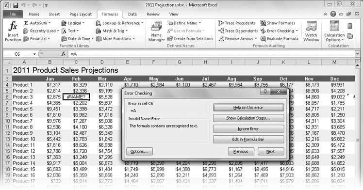
Figure 8-52. The Error Checking dialog box helps you figure out what’s wrong with formulas that display error values.

When a problem appears in the dialog box, the following selections are available:

Click the Previous and Next buttons to locate additional errors on the current worksheet. Click the Options button to display the Formulas category in the Excel Options dialog box, shown in Figure 8-53. Select or clear the check boxes in the two Error Checking areas to determine the type of errors to look for and the way they are processed. Click the Reset Ignored Errors button if you want to recheck or if you clicked the Ignore Error button in the Error Checking dialog box by mistake.

Figure 8-53. Click Options in the Error Checking dialog box to specify error-checking rules.

Sometimes it’s difficult to tell what’s going on in a complex nested formula. A formula is nested when parts of it (called arguments) can be calculated separately. For example, in the formula =IF(Pay_Num<>“”,Scheduled_Monthly_Payment,“”), the named reference Pay_Num indicates a cell that must contain a value in order for the rest of the formula to function. To make this formula easier to read, you can replace this expression with a constant—in this case, 1 (indicating that the expression is TRUE). The formula would then be =IF(1<>“”,Scheduled_Monthly_Payment,“”).

When you click the Evaluate Formula button on the Formulas tab, you can resolve each nested expression one at a time in complex formulas. Figure 8-54 shows the Evaluate Formula dialog box in action.

Click Evaluate to replace each calculable argument with its resulting value. You can click Evaluate as many times as necessary, depending on how many nested levels exist in the selected formula. For example, if you click Evaluate in Figure 8-54, Excel replaces the aforementioned Pay_Num reference with its value. Clicking Evaluate again calculates the next level, and so on, until you reach the end result, which in this case is $188.71, as shown in Figure 8-55.

Figure 8-54. Click the Evaluate Formula button on the Formulas tab to systematically inspect nested formulas.

Figure 8-55. Each time you click the Evaluate button, Excel calculates another nested level in the selected formula.

Eventually, clicking Evaluate results in the formula’s displayed value, and the Evaluate button changes to Restart, letting you repeat the steps. Click Step In to place each calculable reference into a separate box, making the hierarchy more apparent. In our example, the first evaluated reference is to a cell range, which cannot be further evaluated. If the reference is to a cell containing another formula, its address appears in the Evaluate Formula dialog box, as shown in Figure 8-56. Where there are no more steps to be displayed, click Step Out to close the Step In box and replace the reference with the resulting value.

Figure 8-56. Use Step In and Step Out to display calculable arguments separately.

Sometimes you might want to keep an eye on a formula as you make changes to other parts of a worksheet, or even when you’re working on other workbooks that supply information to a worksheet. Instead of constantly having to return to the formula’s location to see the results of your ministrations, you can use the Watch Window, which provides remote viewing for any cell on any open worksheet.

Select a cell you want to keep an eye on, and click Watch Window on the Formulas tab. Then click Add Watch in the Watch Window, as shown in Figure 8-57.

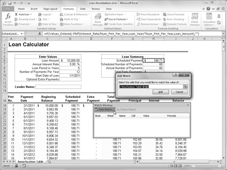
Figure 8-57. Select a cell, and click Watch Window to keep an eye on the cell, no matter where you are currently working.

You can click a cell you want to watch either before or after you display the Add Watch dialog box. Click Add to insert the cell information in the Watch Window. You can dock the Watch Window, as shown in Figure 8-58. You can change its size by dragging its borders or drag it away from its docked position.

While your workbook is still open, you can select any item in the Watch Window list and delete it by clicking Delete Watch. The Watch Window button is a toggle—click it again to close the window; or click the Close button at the top of the Watch Window. When you close a workbook, Excel removes any watched cells the workbook contains from the Watch Window list.

Figure 8-58. The Watch Window displays all the current information for the watched formula.

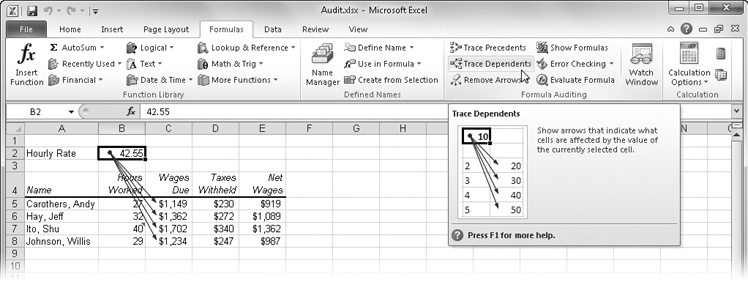
In the worksheet in Figure 8-59, we selected cell B2, which contains an hourly rate value. To find out which cells contain formulas that use this value, click the Trace Dependents button on the Formulas tab. Although this worksheet is elementary to make it easier to illustrate cell tracers, consider the ramifications of using cell tracers in a large and complex worksheet.

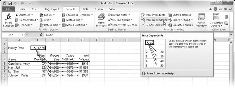
The tracer arrows indicate that cell B2 is directly referred to by the formulas in cells C5, C6, C7, and C8. If you click Trace Dependents again, another set of arrows appears, indicating the next level of dependencies—or indirect dependents. Figure 8-60 shows the results.

One handy feature of the tracer arrows is that you can use them to navigate, which can be advantageous in a large worksheet. For example, in Figure 8-60, with cell B2 still selected, double-click the arrow pointing from cell B2 to cell C8. The selection jumps to the other end of the arrow, and cell C8 becomes the active cell. Now, if you double-click the arrow pointing from cell C8 to cell E8, the selection jumps to cell E8. If you double-click the same arrow again, the selection jumps back to cell C8. If you double-click an arrow that extends beyond the screen, the window shifts to display the cell at the other end. You can use this feature to jump from cell to cell along a path of precedents and dependents.

Figure 8-59. When you trace dependents, arrows point to formulas that directly refer to the selected cell.

Figure 8-60. When you click Trace Dependents again, arrows point to the next level of formulas, ones that indirectly refer to the selected cell.

As you trace precedents or dependents, your screen quickly becomes cluttered, making it difficult to discern the data flow for particular cells. To remove all the tracer arrows from the screen, click the Remove Arrows button in the Formula Auditing group. Alternatively, you can click the small downward-pointing arrow next to the Remove Arrows button to display the Remove Arrows menu, where you can be more selective by choosing Remove Precedent Arrows or Remove Dependent Arrows.

You can also trace in the opposite direction by starting from a cell that contains a formula and tracing the cells that are referred to in the formula. In Figure 8-61, we selected cell E5, which contains one of the net wages formulas, and then clicked Trace Precedents twice to show the complete precedent path.

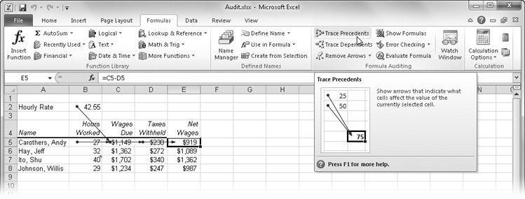
Figure 8-61. When you trace precedents, arrows point from all the cells to which the formula in the selected cell directly refers.

This time, arrows appear with dots in cells B2, B5, C5, and D5, indicating that all these cells are precedents to the selected cell. Notice that the arrows still point in the same direction—toward the formula and in the direction of the data flow—even though we started from the opposite end of the path.

Suppose your worksheet displays error values like the ones shown in Figure 8-62. To trace one of these errors to its source, select a cell that contains an error, and click Trace Error, located on the Error Checking menu in the Formula Auditing group on the Formulas tab. (Refer to Figure 8-52 on page 262.)

Figure 8-62. Cells with error values display an action menu.

Notice that the cells containing errors display small, green, triangular indicators in their upper-left corners, as shown in Figure 8-62, and when you select one of these cells, a floating Trace Error button appears. Clicking the button displays a menu of applicable actions, including Trace Error, a command you can also find on the menu that appears when you click the arrow to the right of the Error Checking button on the Formulas tab, as shown in Figure 8-63.

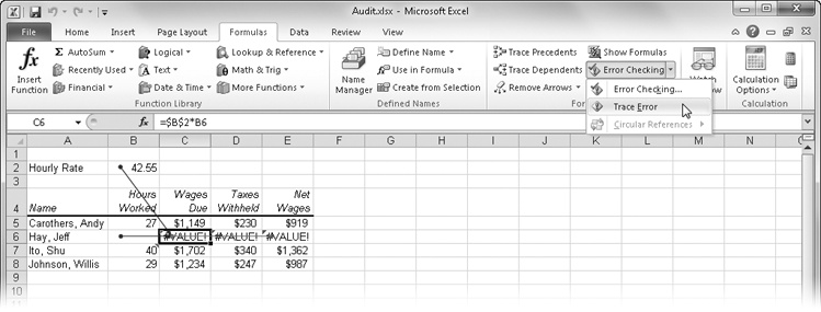
Figure 8-63. Select a cell that contains an error value, and click Trace Error to display arrows that trace the error to its source.

When you click Trace Error, Excel selects the cell that contains the first formula in the error chain and draws red arrows from that cell to the cell you selected, as you can see in Figure 8-63. Excel draws blue arrows to the cell that contains the first erroneous formula from the values the formula uses. It’s up to you to determine the reason for the error; Excel takes you to the source formula and shows you the precedents. In our example, the error is caused by a space character inadvertently entered in cell B6, replacing the hours-worked figure. This is a common, vexing problem because cells containing space characters appear to be empty, but a truly empty cell would not have produced an error in this case.

If a cell contains a reference to a different worksheet or to a worksheet in another workbook, a dashed tracer arrow appears with a small icon attached, as shown in Figure 8-64. You cannot continue to trace precedents using the same procedure from the active cell when a dashed tracer arrow appears.

Figure 8-64. If you trace the precedents of a cell that contains a reference to another worksheet or workbook, a special tracer arrow appears.

If you double-click a dashed tracer arrow, the Go To dialog box appears, with the reference displayed in the Go To list. You can select the reference in the list and click OK to activate the worksheet or workbook. However, if the reference is to a workbook that is not currently open, an error message appears.

After you’ve added text to your comments, nothing is set in stone. You can work with comments using the buttons in the Comments group on the Review tab:

To print comments, follow these steps: