
Many typical spreadsheet models are built in a hierarchical fashion. For example, in a monthly sales worksheet, you might have a column for each month of the year, followed by a totals column, which depends on the numbers in the month columns. You can set up the rows of data hierarchically, with groups of expense categories contributing to category totals. Excel can turn worksheets of this kind into outlines.
Figure 8-66 shows a table of sales figures before outlining, and Figure 8-67 shows the same worksheet after outlining. To accomplish this, we selected cell B3 in the table (any cell would do), clicked the Group menu on the Data tab, and clicked Auto Outline, as shown in Figure 8-66. (To outline a specific range, select the area before choosing Auto Outline.) Figure 8-67 shows how you can change the level of detail displayed after you outline a worksheet.


Figure 8-68 shows the outlined worksheet with columns and rows of detail data hidden simply by clicking all the “minus sign” icons. Without outlining, you would have to hide each group of columns and rows manually; with outlining, you can collapse the outline to change the level of detail instantly.
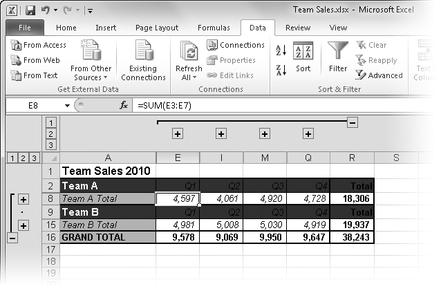
Figure 8-68. Two clicks transformed the outlined worksheet in Figure 8-67 into this quarterly overview.
Tip
Note that after you use the Auto Outline command, you cannot use the Undo command to revert your worksheet to its original state. This is one of the few things within Excel that you can’t undo. Instead, click Clear Outline on the Data tab’s Ungroup menu to remove the outline, which is a better method anyway because you can do it anytime. Interestingly, after you use the Group command—the other command on the Group menu—Undo works just fine.
The standard outline settings reflect the most common worksheet layout. To change these settings, click the dialog box launcher (the little icon to the right of the group name) in the Outline group on the Data tab to display the Settings dialog box shown in Figure 8-69. If your worksheet layout is not typical, such as a worksheet constructed with rows of SUM formulas (or other types of summarization formulas) in rows above the detail rows or with columns of formulas to the left of detail columns, clear the appropriate Direction check box—Summary Rows Below Detail or Summary Columns To Right Of Detail—before outlining.
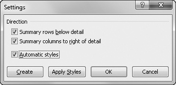
When you use nonstandard worksheet layouts, be sure the area you want to outline is consistent to avoid unpredictable and possibly incorrect results; that is, be sure all summary formulas appear in the same direction relative to the detail data. After you select or clear one or both Direction options, click the Create button to create the outline.
At times, you might create an outline and then add more data to your worksheet. You might also want to re-create an outline if you change the organization of a specific worksheet area. To include new columns and rows in your outline, repeat the procedure you followed to create the outline in the first place: Select a cell in the new area, and click Auto Outline.
Tip
INSIDE OUT Just Say No to Automatic Styles
In the Settings dialog box, the Automatic Styles check box and the Apply Styles button apply rudimentary font formats to your outline that help distinguish totals from detail data. Unfortunately, this isn’t very effective. To ensure that the outline is formatted the way you want, you should plan to apply formats manually.
When you outline a worksheet, Excel displays symbols above and to the left of the row and column headings (refer to Figure 8-67). These symbols take up screen space, so if you want to suppress them, you can click the File tab, Options; then click the Advanced category, and clear the Show Outline Symbols If An Outline Is Applied check box in the Display Options For This Worksheet area. However, this makes it harder to tell whether there is an outline present on the worksheet.


When you create an outline, the areas above and to the left of your worksheet are marked by one or more brackets that terminate in hide detail symbols, which have minus signs on them. The brackets are called level bars. Each level bar indicates a range of cells that share a common outline level. The hide detail symbols appear above or to the left of each level’s summary column or row. If you have hidden the outline symbols or if you prefer to use the ribbon, you can also use the Show Detail and Hide Detail buttons in the Outline group on the Data tab to collapse and expand your outline.
To collapse an outline level so that only the summary cells show, click that level’s hide detail symbol. For example, if you no longer need to see the sales numbers for January through November in the outlined worksheet (refer to Figure 8-67), click the hide detail symbols above columns E, I, and M. The worksheet then looks like Figure 8-70.
Show detail symbols with a plus sign on them now replace the hide detail symbols above the Q1, Q2, and Q3 columns (columns E, I, and M). To redisplay the hidden details, click the show detail symbols.
To collapse each quarter so that only the quarterly totals and annual totals appear, you can click the hide detail symbols above Q1, Q2, Q3, and Q4. The level symbols—the squares with numerals at the upper-left corner of the worksheet—provide an easier way, however. An outline usually has two sets of level symbols, one for columns and one for rows. The column level symbols appear above the worksheet, and the row level symbols appear to the left of the worksheet.
You can use the level symbols to set an entire worksheet to a specific level of detail. The outlined worksheet shown in Figure 8-67 has three levels each for columns and for rows. By clicking both of the level symbols labeled 2 in the upper-left corner of the worksheet, you can transform the outline shown in Figure 8-67 to the one shown in Figure 8-68.
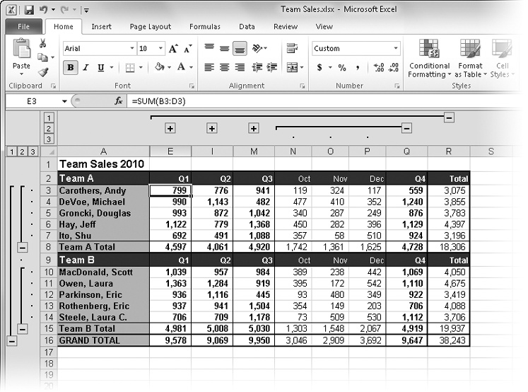
Figure 8-70. When you click the hide detail symbols (–) above Q1, Q2, and Q3, Excel replaces them with show detail symbols (+).
Tip
INSIDE OUT Selecting Only the Visible Cells
When you collapse part of an outline, Excel hides the columns or rows you don’t want to see. In Figure 8-70, for example, the detail columns are hidden for the first three quarters of the year. Ordinarily, if you select a range that includes hidden cells, those hidden cells are implicitly selected. Whatever you do with these cells also happens to the hidden cells, so if you want to copy only the displayed totals, using copy and paste won’t work. Here’s the solution: On the Home tab, click Find & Select, Go To Special, and select the Visible Cells Only option. This is ideal for copying, charting, or performing calculations on only those cells that occupy a particular level of your outline. This feature works the same way in worksheets that have not been outlined; it excludes any cells in hidden columns or rows from the current selection.
If the default automatic outline doesn’t give you the structure you expect, you can adjust it by ungrouping or grouping particular columns or rows. You can easily change the hierarchy of outlined columns and rows by clicking the Group and Ungroup buttons on the Data tab.
For example, you could select row 8 in the outlined worksheet shown in Figure 8-67 and click Ungroup to change row 8 from level 2 to level 1. The outlining symbol to the left of the row moves to the left under the row level symbol labeled 1. To restore the row to its proper level, click Group.
Note
You cannot ungroup or group a nonadjacent selection, and you cannot ungroup a selection that’s already at the highest hierarchical level. If you want to ungroup a top-level column or row to a higher level so that it appears to be separate from the remainder of the outline, you have to group all the other levels of the outline instead.