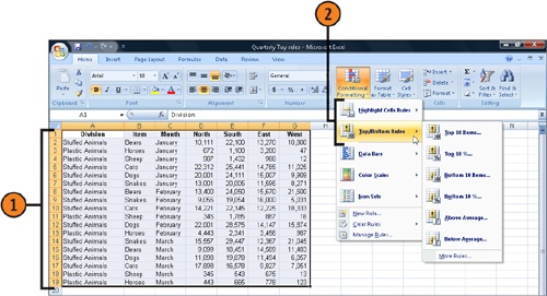
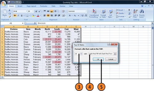
When you use conditional formatting, you can tell Excel to apply specific formatting to any cells that meet the specific criteria you’ve set. For example, you can tell Excel to format a cell whenever the number of sales falls below a certain minimum or whenever the cost rises above a certain figure. Excel will apply the cell formatting only when the conditions you set are found to be true.

Set the Conditional Formatting

1. Select the cells, columns, or rows to which the formatting will apply.

2. On the Home tab, click the Conditional Formatting button, point to Highlight Cells Rules or Top/Bottom Rules, and, in the gallery that appears, click the item you want.

3. Enter the value or values to use for the evaluation.

4. Specify the formatting you want.

5. Click OK.

   
   

Tip

You can apply multiple conditions and formatting to a selection of cells. Make sure, however, that you use different formatting for each criterion so that you’re able to distinguish the different conditions.