For this recipe, we will use the rgl package, so we must first install and load it:

install.packages("rgl")
library(rgl)

We will only use the inbuilt volcano dataset, so we need not load any other dataset.

Let's make a simple three-dimensional surface plot showing the terrain of the Maunga Whau volcano:

z <- 2 * volcano
x <- 10 * (1:nrow(z))
y <- 10 * (1:ncol(z))

zlim <- range(z)
zlen <- zlim[2] - zlim[1] + 1

colorlut <- terrain.colors(zlen) 
col <- colorlut[ z-zlim[1]+1 ] 

rgl.open()
rgl.surface(x, y, z, color=col, back="lines")

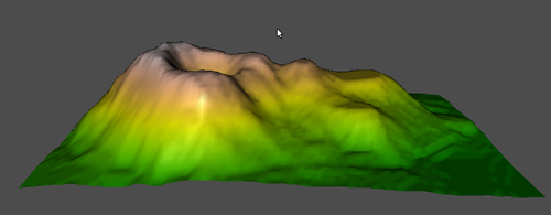
The 3D surface will look like following:

RGL is a 3D real-time rendering device driver system for R. We used the rgl.surface() function to create the preceding visualization. Please see the help section (by running ?rgl.surface at the R prompt) to see the original example at the bottom of the help file, on which the example is based.

We basically used the volcano dataset that we used in the previous couple of recipes and created a three-dimensional representation of the volcano's topography instead of the two-dimensional contour representation.

We set up the x, y, and z arguments in a similar way to the contour examples, except that we multiplied the volcano height data in z by 2 to exaggerate the terrain which helped us appreciate the library's 3D capabilities better.

Then we defined a matrix of colors for each point in z such that each height value has a unique color from the terrain.colors() function. We saved the mapped color data in col (if you type col at the R prompt and hit Return (or Enter), you will see that it contains 5,307 colors).

Then we opened a new RGL device with the rgl.open() command. This brings up a blank window with a gray background. Finally, we called the rgl.surface() function with the x, y, z, and color arguments. We also set the back argument to "lines", which resulted in a wire-framed polygon underneath the visualization.

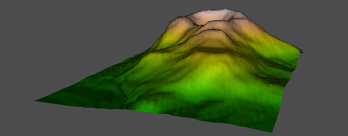
Once rgl.surface() is run, we can rotate the visualization using our mouse in any direction. This lets us look at the volcano from any angle. If we look underneath, we can also see the wire-frame. The images show snapshots of the volcano from four different angles.

The example is a very basic demonstration of the rgl package's functionality.

There are a number of other functions and settings we can use to create a lot more complex visualizations customized to our needs. For example, the back argument can be set to other values to create a filled, point, or hidden polygon. We can also set the transparency (or opacity) of the visualization using the alpha argument. Arguments controlling the appearance of the visualization are sent to the rgl.material() function which sets the material properties.

Please read the related help sections (?rgl, ?rgl.surface, ?rgl.material) to get a more in-depth understanding of this library.