We will use the base graphics library for this recipe, so all you need to do is run the recipe at the R prompt. It is good practice to save your code as a script to use again later.

Once again we will use the cityrain.csv example dataset that we used in Chapter 1 and Chapter 2.

rain<-read.csv("cityrain.csv")
plot(rain$Tokyo,type="b",lwd=2,
xaxt="n",ylim=c(0,300),col="black",
xlab="Month",ylab="Rainfall (mm)",
main="Monthly Rainfall in major cities")
axis(1,at=1:length(rain$Month),labels=rain$Month)
lines(rain$Berlin,col="red",type="b",lwd=2)
lines(rain$NewYork,col="orange",type="b",lwd=2)
lines(rain$London,col="purple",type="b",lwd=2)

legend("topright",legend=c("Tokyo","Berlin","New York","London"),
lty=1,lwd=2,pch=21,col=c("black","red","orange","purple"),
ncol=2,bty="n",cex=0.8,
text.col=c("black","red","orange","purple"),
inset=0.01)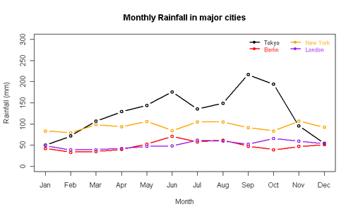

We used the legend() function, which we have already come across in earlier chapters. It is quite a flexible function and allows us to adjust the placement and styling of the legend in many ways.

The first argument we passed to legend() specifies the position of the legend within the plot region. We used "topright"; other possible values are "bottomright", "bottom", "bottomleft", "left", "topleft", "top", "right", and "center". We can also specify the location of legend with x and y co-ordinates as we will soon see.

The other important arguments specific to lines are lwd and lty which specify the line width and type drawn in the legend box respectively. It is important to keep these the same as the corresponding values in the plot() and lines() commands. We also set pch to 21 to replicate the type="b" argument in the plot() command. cex and text.col set the size and colors of the legend text. Note that we set the text colors to the same colors as the lines they represent. Setting bty (box type) to "n" ensures no box is drawn around the legend. This is good practice as it keeps the look of the graph clean. ncol sets the number of columns over which the legend labels are spread and inset sets the inset distance from the margins as a fraction of the plot region .

Let's experiment by changing some of the arguments discussed:

legend(1,300,legend=c("Tokyo","Berlin","New York","London"),
lty=1,lwd=2,pch=21,col=c("black","red","orange","purple"),
horiz=TRUE,bty="n",bg="yellow",cex=1,
text.col=c("black","red","orange","purple"))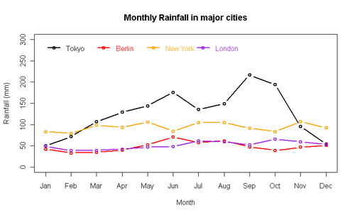

This time we used x and y co-ordinates instead of a keyword to position the legend. We also set the horiz argument to TRUE. As the name suggests, horiz makes the legend labels horizontal instead of the default vertical. Specifying horiz overrides the ncol argument. Finally, we made the legend text bigger by setting cex to 1 and did not use the inset argument.

An alternative way of creating the previous plot without having to call plot() and lines() multiple times is to use the matplot() function. To see details on how to use this function, please see the help file by running ?matplot or help(matplot) at the R prompt.

Have a look at the next recipe, which shows a way to label lines directly instead of using a legend.