In this recipe, we will use the browsers.txt example dataset, which contains data about the usage percentage share of different internet browsers.

First we will load the browsers.txt dataset and then use the pie() function to draw a pie chart:

browsers<-read.table("browsers.txt",header=TRUE)
browsers<-browsers[order(browsers[,2]),]

pie(browsers[,2],
labels=browsers[,1],
clockwise=TRUE,
radius=1,
col=brewer.pal(7,"Set1"),
border="white",
main="Percentage Share of Internet Browser usage")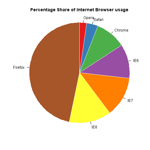

The important thing about the graph is that the slices are ordered in ascending order of their sizes. We have done this because one of the main criticisms of pie charts is that when there are many slices and they are in a random order, it is not easy (often impossible) to tell whether one slice is bigger than another. By ordering the slices by size in a clockwise direction, we can directly compare the slices.

We ordered the dataset by using the order() function, which returns the index of its argument in ascending order. So if we just type order(browsers[,2]) at the R prompt we get:

[1] 7 6 5 3 2 1 4

That's a vector of the index of the share values in ascending order in the original dataset. For example, Firefox which has the largest share is in the fourth row, so the last number in the vector is 4. We then use the index to reassign the browser dataset in the ascending order of share by using the square bracket notation.

Then we pass the share values in the second column as the first argument to the pie() function of the base R graphics library. We set labels to the first column, the names of browsers (note IE stands for Internet Explorer). We also set the clockwise argument to TRUE. By default slices are drawn counterclockwise.

In the next two recipes, we will see how we can further enhance pie charts with percentage value labels.