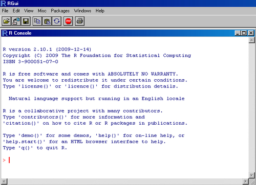
All you need to do to get started is start R. You should have the R prompt on your screen as shown in the following screenshot:

Let's use one of R's inbuilt datasets called cars to look at the relationship between the speed of cars and the distances taken to stop (recorded in the 1920s).

To make your first scatter plot, type the following command at the R prompt:

plot(cars$dist~cars$speed)

This should bring up a window with the following graph showing the relationship between the distance travelled by cars plotted with their speeds:

Now, let's tweak the graph to make it look better. Type the following code at the R prompt:

plot(cars$dist~cars$speed, # y~x
main="Relationship between car distance & speed", # Plot Title
xlab="Speed (miles per hour)", #X axis title
ylab="Distance travelled (miles)", #Y axis title
xlim=c(0,30), #Set x axis limits from 0 to 30
ylim=c(0,140), #Set y axis limits from 0 to 140
xaxs="i", #Set x axis style as internal
yaxs="i", #Set y axis style as internal 
col="red", #Set the color of plotting symbol to red
pch=19) #Set the plotting symbol to filled dots

This should produce the following result:

R comes preloaded with many datasets. In the example, we used one such dataset called cars, which has two columns of data, with the names speed and dist. To see the data, simply type cars at the R prompt and press Enter:

>cars
   speed  dist
1      4     2
2      4    10
3      7     4
4      7    22
. . .
47    24    92
48    24    93
49    24   120
50    25    85
>

As the output from the R command line shows, the cars dataset has two columns and 50 rows of data.

The plot() command is the simplest way to make scatter plots (and other types of plots as we'll see in a moment).

In the first example, we simply pass the x and y arguments that we want to plot in the form plot(y~x) that is, we want to plot distance versus speed. This produces a simple scatter plot. In the second example, we pass a few additional arguments that provide R with more information on how we want the graph to look.

The main argument sets the plot title, xlab and ylab set the X and Y axes titles respectively, xlim and ylim set the minimum and maximum values of the labels on the X and Y axes respectively, xaxs and yaxs set the style of the axes, col and pch set the scatter plot symbol color and type respectively. All of these arguments and more will be explained in detail in Chapter 2, Beyond the Basics.

Instead of the plot(y~x) notation used in the preceding examples, you can also use plot(x,y). For more details on all the arguments the plot() command can take, see the help documentation by typing ?plotor help(plot) at the R prompt, after plotting the first dataset with plot().

If you want to plot another set of points on the same graph, say from another dataset or the same data points but with another symbol on top, you can use the points() function:

points(cars$dist~cars$speed,pch=3)

data()

Scatter plots are covered in a lot more detail in Chapter 3, Creating Scatter Plots.