There’s more to working with your data than organizing the information in worksheets and making it look pretty, and this is where you’ll unleash the real power of Microsoft Office Excel 2007: its ability to make complex statistical, financial, and mathematical computations. In this section, we’ll examine cell notation—the conventions by which Excel references individual cells and ranges of cells—and the way you use cell notation to create formulas that do the calculations for you. We’ll also talk about functions—ready-made bits of code that do the math for you.
There’s some fairly advanced stuff in this section: creating a PivotTable that lets you look at relationships among your data, filtering the data to display items that meet the criteria you specify, troubleshooting formulas, using the AutoFill feature to create a series of calculations, and more. If you’re going to present your data—at a company meeting, for example—the most effective way to do so is with a chart, whose visual appeal holds your audience’s interest more closely than the dry columns and rows of the worksheet on which the chart is based, even though both represent the same data. Excel does more than make your chart look attractive with colors, 3-D effects, and so on—you can plot trendlines to show how your sales figures have improved over time or how your company’s bottom line is on an upward trend.
It’s true that Excel is all about data, but data can include more than just numbers. Excel’s column-and-row format lends itself smoothly to creating and reviewing lists by placing them in tables. Excel provides special features that make short work of sorting your table by specific criteria; filtering it—that is, viewing only part of the list; or summarizing the data in the list.
 In a worksheet, enter the data for your table, making sure that you add descriptive titles for the columns and saving the file as you work.
 In the gallery that appears, click the table style you want to use.
 In the Format As Table dialog box that appears, confirm the range of cells that you want to be included in the table.
 Select this check box if your list has column headings; otherwise, clear the check box if you want Excel to insert generic headings.


See Also
"Excel’s Eccentricities" and "Cell References, Formulas, and Functions" for information about the notation Excel uses to describe ranges of cells.
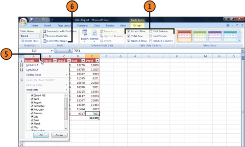
- Click in the table, and, on the Table Tools Design tab, select the check boxes for the items you want displayed and clear the check boxes for the items you don’t want displayed.
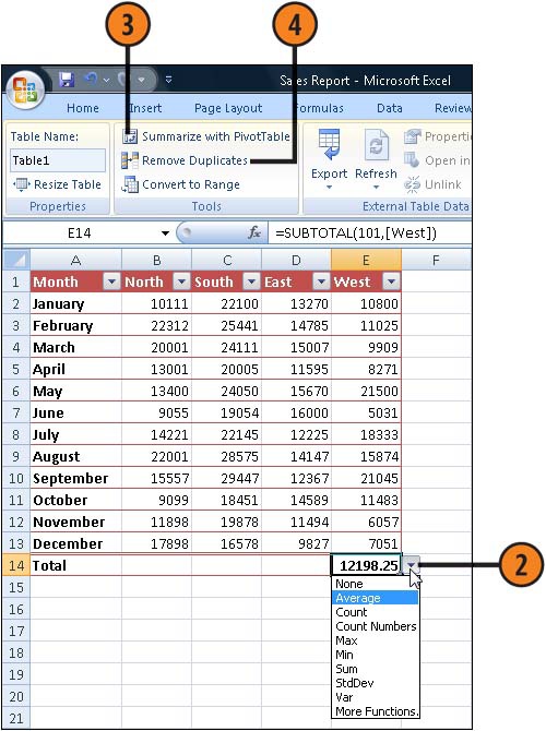
 If you’ve included a totals row, click in the cell that has the totals, click the down arrow that appears, and select the type of total you want. Use the AutoFill feature to copy the totals setting to any other cells that you want to display the total.
 Click Summarize With PivotTable if you want to create a PivotTable based on the data in the table.
- Click Remove Duplicates if you want to remove duplicated information from selected columns.
- Click the down arrow at the top of the column that you want to use to sort or to filter the list; then select the action you want to take. Repeat for any other columns whose data you want to sort or filter.
- Click Convert To Range if you want to convert the table back to standard data in your worksheet.
See Also
"Creating a Series of Calculations" for information about using AutoFill.
"Summarizing the Data with a PivotTable" for information about using a PivotTable to examine your data.