Understanding Cells and Ranges

A cell is a single element in a worksheet that can hold a value, some text, or a formula. A cell is identified by its address or reference, which consists of its column letter and row number. For example, cell D12 is the cell in the fourth column and the twelfth row.

A group of cells is called a range. You designate a range address by specifying its upper-left cell address and its lower-right cell address, separated by a colon.

Here are some examples of range addresses:

C24	A range that consists of a single cell.
A1:B1	Two cells that occupy one row and two columns.
A1:A100	100 cells in column A.
A1:D4	16 cells (four rows by four columns).
C1:C1048576	An entire column of cells; this range also can be expressed as C:C.
A6:XFD6	An entire row of cells; this range also can be expressed as 6:6.
A1:XFD1048576	All cells in a worksheet.

Selecting ranges

To perform an operation on a range of cells in a worksheet, you must first select the range. For example, if you want to make the text bold for a range of cells, you must select the range and then choose Home Font Bold (or press Ctrl+B).

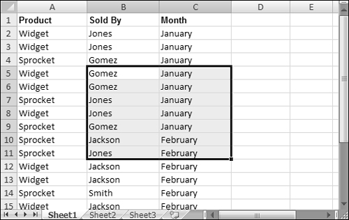
When you select a range, the cells appear highlighted. The exception is the active cell, which remains its normal color. Figure 14-12 shows an example of a selected range (B5:C11) in a worksheet. Cell B5, the active cell, is selected but not highlighted.

You can select a range in several ways:

• Drag diagonally, highlighting the range. If you drag to the end of the screen, the worksheet will scroll.

• Press the Shift key while you use the arrow keys to select a range.

• Press F8 and then move the cell pointer with the arrow keys to highlight the range. Press F8 again to return the arrow keys to normal movement.

• Type the cell or range address into the Name box and press Enter. Excel selects the cell or range that you specified.

• Choose Home Editing Find & Select Go To (or press F5) and enter a range’s address manually into the Go To dialog box. When you click OK, Excel selects the cells in the range that you specified.

Selecting complete rows and columns

Often, you’ll need to select an entire row or column. For example, you may want to apply the same numeric format or the same alignment options to an entire row or column. You can select entire rows and columns in much the same manner as you select ranges:

• Click the row or column border to select a single row or column.

• To select multiple adjacent rows or columns, drag over the row or column borders.

• To select multiple (nonadjacent) rows or columns, press Ctrl while you click the row or column borders that you want.

• Press Ctrl+spacebar to select a column. The column holding the active cell (or columns of the selected cells) is highlighted.

• Press Shift+spacebar to select a row. The row holding the active cell (or rows of the selected cells) is highlighted.

Selecting noncontiguous ranges

Most of the time, the ranges that you select are contiguous—a single rectangle of cells. Excel also enables you to work with noncontiguous ranges, which consist of two or more ranges (or single cells) that aren’t next to each other. Selecting noncontiguous ranges is also known as a multiple selection. If you want to apply the same formatting to cells in different areas of your worksheet, one approach is to make a multiple selection. When the appropriate cells or ranges are selected, the formatting that you select is applied to them all. Figure 14-13 shows a noncontiguous range selected in a worksheet. (Three ranges are selected.)

You can select a noncontiguous range in several ways:

• Select the first range (or cell). Then press Ctrl as you drag the mouse to highlight additional cells or ranges.

• From the keyboard, select a range as described previously (using F8 or the Shift key). Then press Shift+F8 to select another range without canceling the previous range selections.

• Enter the range (or cell) addresses in the Name box, typing a comma between each address. Press Enter.

• Choose Home Editing Find & Select Go To (or press F5) to display the Go To dialog box. Enter the range (or cell) addresses in the Reference box, adding a comma between each range address. Click OK, and Excel selects the ranges.

Selecting multisheet ranges

In addition to two-dimensional ranges on a single worksheet, ranges can extend across multiple worksheets to be three-dimensional ranges.

Suppose that you have a workbook set up to track budgets. A common approach is to use a separate worksheet for each department, making it easy to organize the data. You can click a sheet tab to view the information for a particular department.

Say you have a workbook with four sheets, named Totals, Marketing, Operations, and Manufacturing. The sheets are laid out identically. The only difference is the values. The Totals sheet contains formulas that compute the sum of the corresponding items in the three departmental worksheets.

Assume that you want to apply formatting to the sheets—for example, make the column headings bold with background shading. One (not so efficient) approach is simply to format the cells in each worksheet separately. A better technique is to select a multisheet range and format the cells in all the sheets simultaneously. The following is a step-by-step example of multisheet formatting, using the example workbook described above.

1.	Activate the Totals worksheet by clicking its tab.
2.	Select the range holding the column headings, B3:F3 in the example.
3.	Press Shift and click the sheet tab labeled Manufacturing. This step selects all worksheets between the active worksheet (Totals) and the sheet tab that you click—in essence, a three-dimensional range of cells (see Figure 14-14). Notice that the workbook window’s title bar displays [Group] to remind you that you’ve selected a group of sheets and that you’re in Group edit mode. Figure 14-14. In Group mode, you can work with a three-dimensional range of cells that extends across multiple worksheets.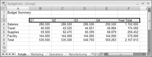 [View full size image]
4.	Choose Home Font Bold and then choose Home Font Fill Color to apply a colored background.
5.	Click one of the other sheet tabs. This step selects the sheet and also cancels Group mode; [Group] is no longer displayed in the title bar. Excel applies the formatting to the selected range across the selected sheets.

When a workbook is in Group mode, any changes that you make to cells in one worksheet also apply to all the other grouped worksheets. You can use this to your advantage when you want to set up a group of identical worksheets because any labels, data, formatting, or formulas you enter are automatically added to the same cells in all the grouped worksheets.

In general, selecting a multisheet range is a simple two-step process: Select the range in one sheet and then select the worksheets to include in the range. To select a group of contiguous worksheets, you can press Shift and click the sheet tab of the last worksheet that you want to include in the selection. To select individual worksheets, press Ctrl and click the sheet tab of each worksheet that you want to select. If all the worksheets in a workbook aren’t laid out the same, you can skip the sheets that you don’t want to format. When you make the selection, the sheet tabs of the selected sheets appear with a white background, and Excel displays [Group] in the title bar.

Selecting special types of cells

As you use Excel, you may need to locate specific types of cells in your worksheets. For example, wouldn’t it be handy to be able to locate every cell that contains a formula—or perhaps all the cells whose value depends on the current cell? Excel provides an easy way to locate these and many other special types of cells. Simply choose Home Select & Find Go To Special to display the Go To Special dialog box, shown in Figure 14-15.

After you make your choice in the dialog box, Excel selects the qualifying subset of cells in the current selection. Usually, this subset of cells is a multiple selection. If no cells qualify, Excel lets you know with the message No cells were found.

Selecting cells by searching

Another way to select cells is to use Excel’s Home Editing Find & Select Find command (or press Ctrl+F), which enables you to select cells by their contents. Click the Options button to display additional choices for refining the search.

Enter the text that you’re looking for; then click Find All. The dialog box expands to display all the cells that match your search criteria. For example, Figure 14-16 shows the dialog box after Excel has located all cells that contain the text Tucson. You can click an item in the list, and the screen will scroll so that you can view the cell in context. To select all the cells in the list, first select any single item in the list. Then press Ctrl+A to select them all.

Note that the Find and Replace dialog box allows you to return to the worksheet without dismissing the dialog box.