Entering and Editing Records

Over time, any list of data requires changes. Most often, the list of items that you’re working with grows over time as you acquire more customers, offer more products, work with more vendors, and so on. Fortunately, the list of data on a worksheet can grow as your needs dictate, and Excel provides a variety of methods for updating and controlling the data in any table.

Using keyboard entry

Plain old keyboard entry, just the same as entering any other worksheet cell data, seems a bit unglamorous and tedious. Still, typing in new records is just part of the bargain when you’re maintaining any list of information.

Whenever you type data into the next blank row below a table that you’ve defined on a worksheet, Excel automatically assumes that you want to add to the table, and so it adjusts the range defined as the table and formats the new record or row using the style applied to the rest of the table. For example, Figure 19-5 shows a new row of data being entered into the table from Figure 19-3.

Figure 19-5. Excel automatically expands the table to encompass any new row you type.

[View full size image]

If you add new row(s) or column(s) of data that aren’t automatically included by Excel, you can expand or resize the table. To do so:

1.	Select Design Properties Resize Table.
2.	Specify the range that holds the old and new table contents using the Select the New Data Range for Your Table text box of the Resize Table dialog box.
3.	Click OK. Excel expands the table to encompass the new range.

Using the data form

Once you’ve established your basic database or table, you can use the data form to delete or edit data in any field of any record. You also can use it to input entirely new records.

As Chapter 13 explained, you have to add a button for the data form to the Quick Access toolbar in order to use the form. You add the button by customizing the Quick Access toolbar. To do so, right-click the toolbar and then click Customize Quick Access toolbar. Select Commands Not in the Ribbon from the Choose Commands from drop-down list, scroll down, click Form, click Add, and then click OK.

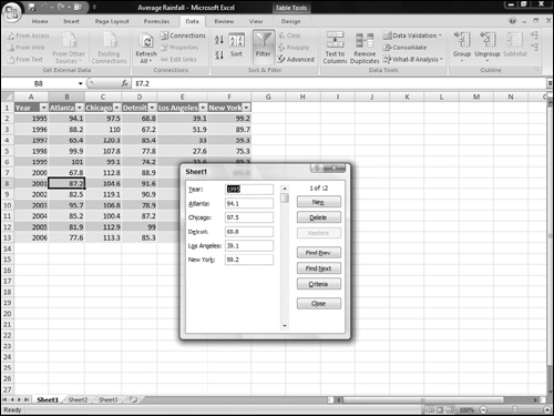
To use the data form, follow these steps:

1.	Select any cell within the list or table. (The list need not be defined as a table. It need only have a header row to identify the name of each field.) This cell can be within a record or within the field labels on the top row, just as long as it’s not outside the list or table.
2.	Click the Form button on the Quick Access toolbar. Figure 19-6 shows this button, and the resulting form that appears. Figure 19-6. You can use this form to add information to a list or table. [View full size image]
3.	Click the down and/or up arrows on the scroll bar to display the desired record, then edit text box (field) entries as desired.
4.	To add a new record, click the New button and then type the new field entries. Tip Pressing the Esc key when no changes have been made will close the form. Tip You can walk through the entire database by repeatedly pressing Enter without entering any new data.
5.	To permanently remove the displayed record, click the Delete button and then click OK in the confirmation message box (Figure 19-7). Figure 19-7. Confirm that you want to delete the record, when prompted.
6.	Click Close to close the form dialog box when you finish. Caution When you delete a record from the database with the form’s Delete button, the warning message isn’t kidding about its being permanently gone. You can’t even use Undo to reverse the action the way you can with other actions.

Data validation parameters

As in prior versions, Excel 2007 enables you to set up data validation that you can use to ensure that accurate values are entered in a list or table. For example, you can specify that a field can only hold a whole number between two other values, or a date after a particular point in time.

To set values and parameters for data validation, follow these steps:

1.	Click the column heading (column letter) for the field you want to apply the data validation to.
2.	Select Data Data Tools Data Validation from the Ribbon.
3.	Click the Settings tab in the Data Validation dialog box (see Figure 19-8). Figure 19-8. This dialog box enables you to specify what entries are “legal” for a table field.
4.	Choose from one of the values under Allow (for a description of these values, see Table 19-1). Table 19-1. Value Settings for Data Validation Allowed Value Meaning Any Value No restrictions Whole Number Restricted to numbers without decimals Decimal Restricted to numbers, but allows decimals List Restricted to a preset list of options Date Restricted to calendar data Time Restricted to clock data Text Length Restricted to specified length Custom Restricted to custom formula
5.	Choose from one of the options under Data (described in Table 19-2). The Data field is disabled for some of the Allow options. Table 19-2. Options for Data Validation Values Option Meaning Between The value must fall between minimum and maximum values. Not between The value must not be between the specified values. Equal to The value must be the same as the specified value. Not equal to The value must not be the specified value. Greater than The value must be more than the specified value. Less than The value must be less than the specified value. Greater than or equal to The value must be the same as or more than the specified value. Less than or equal to The value must be the same as or less than the specified value.
6.	The parameters displayed depend on the options chosen under Allow and Data. Enter the parameters for the restrictions. In many cases, these are simply minimum and/or maximum values, such as the lowest and highest numbers or the earliest and latest dates allowed.
7.	Click the OK button to finish.

List, text length, and custom values

Three of the value options listed in Table 19-1 require further explanation. The List option draws from a predefined list of values. You can type them in directly under Source (separated by commas), or you can specify a range of cells in that space that contain the list of acceptable entries. Text length, despite the name, does not require that it be applied to text. You can also specify the length of a number with it. (In other words, you can specify the number of digits in a number.) The Custom setting limits the entry to anything that fits a formula you’ve designed. As with the List parameters, you can either type it in directly (under Formula), or specify a cell reference that contains the formula.

Error messages

Any time you set validation parameters (anything other than All Values), an error message will be generated if inappropriate values are entered. The default error message has a title of simply “Microsoft Excel” and is so general as to be virtually meaningless—”The value you entered is not valid. A user has restricted values that can be entered into this cell.” To change this, follow these steps:

1.	Select the column heading for the field you want to create an error message for.
2.	Select Data Data Tools Data Validation from the Ribbon.
3.	Click the Error Alert tab (see Figure 19-9). Figure 19-9. Set up validation error messages on this tab.
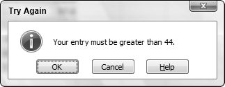
4.	Choose the desired type of warning from the Style drop-down list: Stop, Warning, and Information. Stop is the default, and presents a red circle with a white X in the middle of it when an error occurs. Warning shows a yellow triangle with a black exclamation point in the middle, and Information shows a dialog balloon with a blue “i” in the middle. Each of the three gives you the option to enter the title and text of the error message, or both. If you do not specify one of them, it will remain at the default setting. The three differ as follows: The Stop error message presents Retry and Cancel buttons (see Figure 19-10). The effect of both is identical, with only a small technical difference. The Retry button highlights the erroneous entry, meaning that anything you type will replace it. The Cancel button deletes the erroneous entry, also leaving you free to type a new one. Figure 19-10. The Stop error message. The Warning error message presents three options: Yes, No, and Cancel buttons (see Figure 19-11). Clicking the Yes button enters the erroneous value even though it’s supposed to be excluded. Clicking the No button is identical to clicking the Retry button for the Stop error message—it highlights the erroneous entry so you can type a new one. The Cancel button, once again, simply deletes the erroneous entry and leaves the cell selected, so you can type a new entry if you want to or move on. Figure 19-11. The Warning error message. The Information error message presents only OK and Cancel buttons (see Figure 19-12). Clicking the OK button enters the erroneous value, whereas clicking the Cancel button deletes the erroneous entry and leaves the cell selected. Figure 19-12. The Information error message.
5.	Click the OK button to complete the process.

Cell input messages

Cell input messages are not an integral part of the data-validation process but a fairly frivolous add-on. These messages are displayed whenever a cell containing them is selected. Although they can be used to say things like, “Enter such and such a value in this cell,” the purpose of the cell should already be obvious from the field label. If it isn’t, give some serious thought to rewriting your field labels.

In actual practice, cell input messages have limited utility and tend mainly to simply obscure part of the database from view. If you must use them, use them sparingly, or you will find that they make the database totally unworkable. However, in some cases they can serve to help bullet-proof your worksheets, as in the example in Figure 19-13.

To create a cell input message, follow these steps:

1.	Select either the column heading for the field or the individual cell you want to apply the data validation to.
2.	Select Data Data Tools Data Validation from the Ribbon.
3.	Click the Input Message tab.
4.	Enter the Title and Input Message text for the error message. If you do not specify the text, no message will appear, even if you do specify a title. If you do specify a title, the title will show in the first line of the message in bold print.
5.	Click the OK button to complete the process.