
Modifying Cell Contents
After you enter a value or text into a cell, you can modify it in several ways:
Erase the cell’s contents
Replace the cell’s contents with something else
Edit the cell’s contents
Erasing the contents of a cell
To erase the contents of a cell, just click the cell and press Delete. To erase more than one cell, select all the cells that you want to erase and then press Delete. Pressing Delete removes the cell’s contents but doesn’t remove any formatting (such as bold, italic, or a different number format) that you may have applied to the cell.
For more control over what gets deleted, you can choose Home ![]() Editing
Editing ![]() Clear. This command’s drop-down list has four choices:
Clear. This command’s drop-down list has four choices:
Clear All: Clears everything from the cell
Clear Formats: Clears only the formatting and leaves the value, text, or formula
Clear Contents: Clears only the cell’s contents and leaves the formatting
Clear Comments: Clears the comment (if one exists) attached to the cell
Note
Clearing formats doesn’t clear the background colors in a range that has been designated as a table, unless you’ve replace the table style background colors manually.
Replacing the contents of a cell
To replace the contents of a cell with something else, just activate the cell and type your new entry, which replaces the previous contents. Any formatting that you previously applied to the cell remains in place and is applied to the new content.
Tip
You can also replace cell contents by dragging and dropping or by pasting data from the Clipboard. In both cases, the cell formatting will be replaced by the format of the new data. To avoid pasting formatting, choose Home ![]() Clipboard
Clipboard ![]() Paste and select Formulas or Paste Values.
Paste and select Formulas or Paste Values.
Editing the contents of a cell
If the cell contains only a few characters, replacing its contents by typing new data usually is easiest. But if the cell contains lengthy text or a complex formula and you need to make only a slight modification, you probably want to edit the cell rather than re-enter information.
When you want to edit the contents of a cell, you can use one of the following ways to enter cell-edit mode:
Double-clicking the cell enables you to edit the cell contents directly in the cell.
Selecting the cell and pressing F2 enables you to edit the cell contents directly in the cell.
Selecting the cell that you want to edit and then clicking inside the Formula bar enables you to edit the cell contents in the Formula bar.
You can use whichever method you prefer. Some people find editing directly in the cell easier; others prefer to use the Formula bar to edit a cell.
Note
The Advanced tab of the Excel Options dialog box contains a section called Editing Options. These settings affect how editing works. (To access this dialog box, choose Office Button ![]() Excel Options.) If the option labeled Allow Editing Directly In Cells isn’t enabled, you aren’t able to edit a cell by double-clicking. In addition, pressing F2 allows you to edit the cell in the Formula bar (not directly in the cell).
Excel Options.) If the option labeled Allow Editing Directly In Cells isn’t enabled, you aren’t able to edit a cell by double-clicking. In addition, pressing F2 allows you to edit the cell in the Formula bar (not directly in the cell).
All these methods cause Excel to go into edit mode. (The word Edit appears at the left side of the status bar at the bottom of the screen.) When Excel is in edit mode, the Formula bar displays two new icons: the X and Check Mark (see Figure 13-3). Clicking the X icon cancels editing, without changing the cell’s contents. (Pressing Esc has the same effect.) Clicking the Check Mark icon completes the editing and enters the modified contents into the cell. (Pressing Enter has the same effect.)
Figure 13-3. While editing a cell, the Formula bar displays two new icons.

When you begin editing a cell, the insertion point appears as a vertical bar, and you can move the insertion point by using the arrow keys. Use Home to move the insertion point to the beginning of the cell and use End to move the insertion point to the end. You can add new characters at the location of the insertion point. To select multiple characters, press Shift while you use the arrow keys. You also can use the mouse to select characters while you’re editing a cell. Just click and drag the mouse pointer over the characters that you want to select.
Learning some handy data-entry techniques
You can simplify the process of entering information into your Excel worksheets and make your work go quite a bit faster by using a number of useful tricks, described in the following sections.
Automatically moving the cell pointer after entering data
By default, Excel automatically moves the cell pointer to the next cell down when you press the Enter key after entering data into a cell. To change this setting, choose Office Button ![]() Excel Options and click the Advanced item (see Figure 13-4) in the list at the left. The checkbox that controls this behavior is labeled After Pressing Enter, Move Selection. You can also specify the direction in which the cell pointer moves (down, left, up, or right).
Excel Options and click the Advanced item (see Figure 13-4) in the list at the left. The checkbox that controls this behavior is labeled After Pressing Enter, Move Selection. You can also specify the direction in which the cell pointer moves (down, left, up, or right).
Figure 13-4. You can use the Advanced choices in the Excel Options dialog box to select a number of helpful input option settings.

Your choice is completely a matter of personal preference. I prefer to keep this option turned off. When entering data, I use the arrow keys rather than the Enter key (see the next section).
Using arrow keys instead of pressing Enter
Instead of pressing the Enter key when you’re finished making a cell entry, you also can use any of the directional keys to complete the entry. Not surprisingly, these directional keys send you in the direction that you indicate. For example, if you’re entering data in a row, press the right-arrow (→) key rather than Enter. The other arrow keys work as expected, and you can even use PgUp and PgDn.
Selecting a range of input cells before entering data
Here’s a tip that most Excel users don’t know about: When a range of cells is selected, Excel automatically moves the cell pointer to the next cell in the range when you press Enter. If the selection consists of multiple rows, Excel moves down the column; when it reaches the end of the selection in the column, it moves to the first selected cell in the next column.
To skip a cell, just press Enter without entering anything. To go backward, press Shift+Enter. If you prefer to enter the data by rows rather than by columns, press Tab rather than Enter.
Using Ctrl+Enter to place information into multiple cells simultaneously
If you need to enter the same data into multiple cells, Excel offers a handy shortcut. Select all the cells that you want to contain the data; type the value, text, or formula, which will appear in the formula bar; and then press Ctrl+Enter (instead of Enter). The same information is inserted into each cell in the selection.
Entering decimal points automatically
If you need to enter lots of numbers with a fixed number of decimal places, Excel has a useful tool that works like some adding machines. Open the Excel Options dialog box (Office Button ![]() Excel Options) and click the Advanced choice. Select the checkbox Automatically Insert a Decimal Point and make sure that the Places box is set for the correct number of decimal places for the data you need to enter.
Excel Options) and click the Advanced choice. Select the checkbox Automatically Insert a Decimal Point and make sure that the Places box is set for the correct number of decimal places for the data you need to enter.
When this option is set, Excel supplies the decimal points for you automatically. For example, if you’ve specified two decimal places, entering 12345 into a cell is interpreted as 123.45. To restore things to normal, just uncheck the Automatically Insert a Decimal Point checkbox in the Excel Options dialog box. Changing this setting doesn’t affect any values that you have already entered.
Caution
The fixed-decimal-places option is a global setting and applies to all workbooks (not just the active workbook). If you forget that this option is turned on, you can easily end up entering incorrect values—or some major confusion if someone else uses your computer.
Using AutoFill to enter a series of values
Excel’s AutoFill feature makes inserting a series of values or text items in a range of cells easy. It uses the AutoFill handle (the small box at the lower right of the active cell). You can drag the AutoFill handle to copy the cell or automatically complete a series.
If you drag the AutoFill handle while you press the right mouse button, Excel displays a shortcut menu with additional fill options.
Figure 13-5 shows an example. I entered 1 into cell A1 and 3 into cell A2. Then I selected both cells and dragged the fill handle down to create a linear series of odd numbers.
Figure 13-5. This series was created using AutoFill.

Using AutoComplete to automate data entry
Excel’s AutoComplete feature makes entering the same text into multiple cells easy. With AutoComplete, you type the first few letters of a text entry into a cell, and Excel automatically completes the entry based on other entries that you’ve already made in the column. Besides reducing typing, this feature also ensures that your entries are spelled correctly and are consistent.
Here’s how it works. Suppose that you’re entering product information in a column. One of your products is named Widgets. The first time that you enter Widgets into a cell, Excel remembers it. Later, when you start typing Widgets in that same column, Excel recognizes it by the first few letters and finishes typing it for you. Just press Enter, and you’re done. It also changes the case of letters for you automatically. If you start entering widget (with a lowercase w) in the second entry, Excel makes the w uppercase to be consistent with the previous entry in the column.
Tip
You also can access a mouse-oriented version of AutoComplete by right-clicking the cell and selecting Pick From Drop-Down List from the shortcut menu. Excel then displays a drop-down box that has all the entries in the current column, and you just click the one that you want.
Keep in mind that AutoComplete works only within a contiguous column of cells. If you have a blank row, for example, AutoComplete identifies only the cell contents below the blank row.
If you find the AutoComplete feature distracting, you can turn it off by using the Advanced settings of the Excel Options dialog box. Remove the check mark from the checkbox labeled Enable AutoComplete For Cell Values. (See Appendix A, “Customizing Office,” for more information about changing options.)
Forcing text to appear on a new line within a cell
If you have lengthy text in a cell, you can force Excel to display it in multiple lines within the cell. Use Alt+Enter to start a new line in a cell.
Note
When you add a line break, Excel automatically changes the cell’s format to Wrap Text. But unlike normal text wrap, your manual line break forces Excel to break the text at a specific place within the text, which gives you more precise control over the appearance of the text than if you rely on automatic text wrapping.
Tip
To remove a manual line break, edit the cell and press Delete when the insertion point is located at the end of the line that contains the manual line break. You won’t see any symbol to indicate the position of the manual line break, but the text that follows it will move up when the line break is deleted.
Using AutoCorrect for shorthand data entry
You can use Excel’s AutoCorrect feature to create shortcuts for commonly used words or phrases. For example, if you work for a company named Consolidated Data Processing Corporation, you can create an AutoCorrect entry for an abbreviation, such as cdp. Then, whenever you type cdp, Excel automatically changes it to Consolidated Data Processing Corporation.
Excel includes quite a few built-in AutoCorrect terms (mostly common misspellings), and you can add your own. To set up your custom AutoCorrect entries, access the Excel Options dialog box (choose Office Button ![]() Excel Options) and click the Proofing tab. Then click the AutoCorrect Options button to display the AutoCorrect dialog box. In the dialog box, click the AutoCorrect tab, check the option labeled Replace Text As You Type, and then enter your custom entries. (Figure 13-6 shows an example.) You can set up as many custom entries as you like. Just be careful not to use an abbreviation that might appear normally in your text.
Excel Options) and click the Proofing tab. Then click the AutoCorrect Options button to display the AutoCorrect dialog box. In the dialog box, click the AutoCorrect tab, check the option labeled Replace Text As You Type, and then enter your custom entries. (Figure 13-6 shows an example.) You can set up as many custom entries as you like. Just be careful not to use an abbreviation that might appear normally in your text.
Figure 13-6. AutoCorrect allows you to create shorthand abbreviations for text you enter often.

Tip
Excel shares your AutoCorrect list with other Office applications. For example, any AutoCorrect entries you created in Word also work in Excel.
Entering numbers with fractions
To enter a fractional value into a cell, leave a space between the whole number and the fraction. For example, to enter 6⅞, enter 6 7/8 and then press Enter. When you select the cell, 6.875 appears in the Formula bar, and the cell entry appears as a fraction. If you have a fraction only (for example, ⅛), you must enter a zero first, like this: 0 1/8—otherwise, Excel will likely assume that you’re entering a date. When you select the cell and look at the Formula bar, you see 0.125. In the cell, you see ⅛.
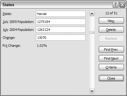
Simplifying data entry by using a form
Many people use Excel to manage lists in which the information is arranged in rows. Excel offers a simple way to work with this type of data through the use of a data entry form that Excel can create automatically. This data form works with either a normal range of data or with a range that has been designated as a table (choosing Insert ![]() Tables
Tables ![]() Table). Figure 13-7 shows an example.
Table). Figure 13-7 shows an example.
Figure 13-7. Excel’s built-in data form can simplify many data-entry tasks.
Unfortunately, the command to access the data form is not in the Ribbon. To use the data form, you must add it to your Quick Access toolbar (QAT):
1. | Right-click the QAT and select Customize Quick Access Toolbar. The Customize panel of the Excel Options dialog box appears. |
2. | In the Choose Commands From drop-down list, select Commands Not In The Ribbon. |
3. | In the list box on the left, select Form. |
4. | Click the Add button to add the selected command to your QAT. |
5. | Click OK to close the Excel Options dialog box. |
After performing these steps, a new button appears on your QAT.
To use a data entry form, you must arrange your data so that Excel can recognize it as a table. Start by entering headings for the columns in the first row of your data entry range. Select any cell in the table and click the Form button on your QAT. Excel then displays a dialog box customized to your data. You can use Tab to move between the text boxes and supply information. If a cell contains a formula, the formula result appears as text (not as an edit box). In other words, you can’t modify formulas using the data entry form.
When you complete the data form, click the New button. Excel enters the data into a row in the worksheet and clears the dialog box for the next row of data.
Entering the current date or time into a cell
If you need to date-stamp or time-stamp your worksheet, Excel provides two shortcut keys that do this task for you:
Current date: Ctrl+; (semicolon)
Current time: Ctrl+Shift+; (semicolon)
Note
When you use either of these shortcuts to enter a date or time into your worksheet, Excel enters a static value into the worksheet. In other words, the date or time entered doesn’t change when the worksheet is recalculated. In most cases, this setup is probably what you want, but you should be aware of this limitation. If you want the date or time display to update, use one of these formulas:
=TODAY()
=NOW()