Using Formulas in Tables

One of the most significant new features in Excel 2007 is its support for tables. In this section I describe how formulas work with tables.

Summarizing data in a table

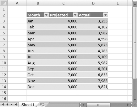
Figure 15-10 shows a simple table with three columns. I entered the data, and then converted the range to a table by choosing Insert Tables Table. Note that I didn’t define any names, but the table is named Table1 by default.

If you’d like to calculate the total projected and total actual sales, you don’t even need to write a formula. Simply click a button to add a row of summary formulas to the table:

1.	Activate any cell in the table.
2.	Place a check mark next to Table Tools Design Table Style Options Total Row.
3.	Activate a cell in the Total Row and use the drop-down list to select the type of summary formula to use (see Figure 15-11). For example, to calculate the sum of the Actual column, select SUM from the drop-down list in cell D15. Excel creates this formula: =SUBTOTAL(109,[Actual]) Figure 15-11. A drop-down list enables you to select a summary formula for a table column. [View full size image]

For the SUBTOTAL function, 109 is an enumerated argument that represents SUM. The second argument for the SUBTOTAL function is the column name, in square brackets. Using the column name within brackets is a new way to create “structured” references within a table. (I discuss this further in an upcoming section, “Referencing data in a table.”)

Using formulas within a table

In many cases, you’ll want to use formulas within a table. For example, in the table shown in Figure 15-11, you may want a column that shows the difference between the Actual and Projected amounts. As you’ll see, Excel 2007 makes this very easy.

Figure 15-12 shows the table with the new column.

Figure 15-12. The Difference column contains a formula.

[View full size image]

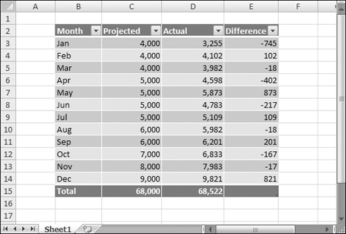
If you examine the table, you’ll find this formula for all cells in the Difference column:

=[Actual]-[Projected]

Although the formula was entered into the first row of the table, that’s not necessary. Any time a formula is entered into an empty table column, it will automatically fill all the cells in that column. And if you need to edit the formula, Excel will automatically copy the edited formula to the other cells in the column.

The steps listed above used the pointing technique to create the formula. Alternatively, you could have entered it manually using standard cell references. For example, you could have entered the following formula in cell E3:

=D3-C3

If you type the cell references, Excel will still copy the formula to the other cells automatically.

One thing should be clear, however, about formulas that use the column headers: They are much easier to understand.

Referencing data in a table

Excel 2007 adds some new ways to refer to data that’s contained in a table by using the table name and column headers. There is no need to create names for these items. The table itself has a name (for example, Table1), and you can refer to data within the table by using column headers.

You can, of course, use standard cell references to refer to data in a table, but the new method has a distinct advantage: The names adjust automatically if the table size changes by adding or deleting rows.

Refer to the table shown in Figure 15-11. This table was given the name Table1 when it was created. To calculate the sum of all the data in the table, use this formula:

=SUM(Table1)

This formula will always return the sum of all the data, even if rows or columns are added or deleted. And if you change the name of Table1, Excel will adjust formulas that refer to that table automatically. For example, if you renamed Table1 to be AnnualData (by using the Name Manager), the preceding formula would be changed to:

=SUM(AnnualData)

Most of the time, you’ll want to refer to a specific column in the table. The following formula returns the sum of the data in the Actual column:

=SUM(Table1[Actual])

Notice that the column name is enclosed in square brackets. Again, the formula adjusts automatically if you change the text in the column heading.

Even better, Excel provides some helpful assistance when you create a formula that refers to data within a table. Figure 15-13 shows formula AutoComplete helping to create a formula by showing a list of the elements in the table.