Controlling the Worksheet View

As you add more information to a worksheet, you may find that navigating and locating what you want gets more difficult. Excel includes a few options that enable you to view your sheet, and sometimes multiple sheets, more efficiently. This section discusses a few additional worksheet options at your disposal.

Zooming in or out for a better view

Normally, everything you see on-screen is displayed at 100 percent. You can change the zoom percentage from 10 percent (very tiny) to 400 percent (huge). Using a small zoom percentage can help you to get a bird’s-eye view of your worksheet to see how it’s laid out. Zooming in is useful if your eyesight isn’t quite what it used to be and you have trouble deciphering tiny type. Zooming doesn’t change the font size, so it has no affect on printed output.

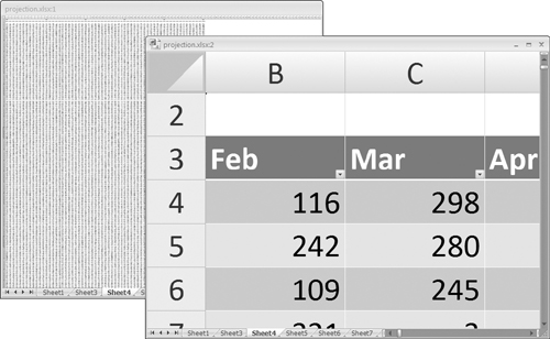
Figure 14-5 shows a window zoomed to 10 percent and a window zoomed to 400 percent.

You can easily change the zoom factor of the active worksheet by using the Zoom slider located on the right end of the status bar. Drag the slider, and your screen transforms instantly.

Another way to zoom is to choose View Zoom Zoom, which displays a dialog box. Choosing View Zoom Zoom To Selection zooms the worksheet to display only the selected cells (useful if you want to view only a particular range).

Viewing a worksheet in multiple windows

Sometimes, you may want to view two different parts of a worksheet simultaneously—perhaps to make referencing a distant cell in a formula easier. To create and display a new view of the active workbook, choose View Window New Window.

Excel displays a new window for the active workbook, similar to the one shown in Figure 14-6. In this case, each window shows a different worksheet in the workbook. Notice the text in the windows’ title bars: climate data.xls:1 and climate data.xls:2. To help you keep track of the windows, Excel appends a colon and a number to each window.

A single workbook can have as many views (that is, separate windows) as you want. Scrolling to a new location in one window doesn’t cause scrolling in the other window(s).

You can close these additional windows when you no longer need them. Clicking the Close button on the active window’s title bar closes the active window but doesn’t close the other windows for the workbook.

Comparing sheets side by side

In some situations, you may want to compare two worksheets that are in different windows. The View Side By Side feature makes this task a bit easier.

First, make sure that the two sheets are displayed in separate windows. (The sheets can be in the same workbook or in different workbooks.) Activate the first window; then choose View Window View Side by Side. If more than two windows are open, you see a dialog box that lets you select the window for the comparison. The two windows appear next to each other.

When using the View Side by Side feature, scrolling in one of the windows also scrolls the other window. If, for some reason, you don’t want this simultaneous scrolling, choose View Window Synchronous Scrolling (which is a toggle). If you have rearranged or moved the windows, choose View Window Reset Window Position to restore the windows to the initial side-by-side arrangement. To turn off the side-by-side viewing, choose View Window View Side by Side again.

Keep in mind that this feature is for manual comparison only. Unfortunately, Excel doesn’t provide a way to show you the differences between two sheets.

Splitting the worksheet window into panes

If you prefer not to clutter your screen with additional windows, Excel provides another option for viewing multiple parts of the same worksheet. Choosing View Window Split splits the active worksheet into two or four separate panes. The split occurs at the location of the cell pointer. If the cell pointer is in row 1 or column A, this command results in a two-pane split. Otherwise, it gives you four panes. You can use the mouse to drag the individual panes to resize them.

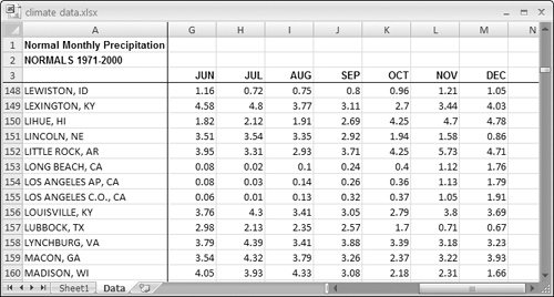
Figure 14-7 shows a worksheet split into two panes. Notice that row numbers aren’t continuous. In other words, splitting panes enables you to display in a single window widely separated areas of a worksheet. To remove the split panes, choose View Window Split again or just double-click on the split bar you want removed.

Keeping the titles in view by freezing panes

If you set up a worksheet with row or column headings, these headings will not be visible when you scroll down or to the right. Excel provides a handy solution to this problem: freezing panes. Freezing panes keeps the headings visible while you’re scrolling through the worksheet.

To freeze panes, start by moving the cell pointer to the cell below the row that you want to remain visible as you scroll vertically, and to the right of the column that you want to remain visible as you scroll horizontally. Then, choose View Window Freeze Panes and select the Freeze Panes option from the drop-down list. Excel inserts dark lines to indicate the frozen rows and/or columns. The frozen area remains visible as you scroll throughout the worksheet. To remove the frozen panes, choose View Window Freeze Panes, and select the Unfreeze Panes option from the drop-down list.

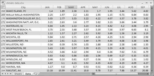
Figure 14-8 shows a worksheet with frozen panes. In this case, rows 1:3 and column A are frozen in place. This technique allows you to scroll down and to the right to locate some information while keeping the column titles and the column A entries visible.

Monitoring cells with a Watch Window

In some situations, you may want to monitor the value in a particular cell as you work. As you scroll throughout the worksheet, that cell may disappear from view. A feature known as Watch Window can help. A Watch Window displays the value of any number of cells in a handy window that’s always visible.

To display the Watch Window, choose Formulas Formula Auditing Watch Window. The Watch Window appears in the task pane, but you can also drag it and make it float over the worksheet.

To add a cell to watch, click Add Watch and specify the cell that you want to watch. The Watch Window displays the value in that cell. You can add any number of cells to the Watch Window, and you can move the window to any convenient location. Figure 14-10 shows the Watch Window monitoring four cells.