Sorting and Filtering Data

The order in which you enter the records in your database doesn’t ultimately matter, because you can sort and filter the table after the fact. Sorting simply changes the order in which the rows or records are displayed, whereas filtering creates a display of only those rows or records that fit criteria you have specified.

Sorting data

The easiest way to sort is to simply select any cell in the column you want to sort by and then click either the Sort Ascending or Sort Descending buttons in the Sort * Filter group of the Data tab on the Ribbon. The Sort Ascending button sorts from A to Z (it’s the one with A on top and Z on the bottom). Technically speaking, it sorts from zero to Z, but that wouldn’t make as good an icon. The Sort Descending button sorts from Z to A (okay, Z to zero), and it’s the one with Z on top and A on the bottom. Figure 19-14 shows data sorted in descending order by year.

The drawback to this method, as with so many things that are simple to use, is that it lacks real power. Often, you’ll find that you need to sort by more than one column. For instance, you might need to sort a customer database by both state and product ordered so you can determine which products are selling best in which states. Or you might want to sort the weather database by year and temperature.

To sort by multiple columns, follow these steps:

1.	Select any cell in the list or table.
2.	Select Data Sort & Filter Sort in the Ribbon. If you failed to select a cell in the database, Excel will tell you it can’t find it. In that case, go back to Step 1.
3.	Specify sort levels in the Sort dialog box (see Figure 19-15). Click the Add Level button to specify each new sort level, then use the Column, Sort On, and Order drop-down lists to specify the field, type of cell information, and sort order for the sort. Figure 19-15. Use this dialog box to set up a more advanced sort. [View full size image]
4.	Click the OK button to apply the sort.

Filtering data

Filtering your data is much more powerful than simply sorting it. Instead of being limited to three columns as you are for a sort, you can filter on any or all columns in your table. Filtering removes from view any record that doesn’t match your criteria (but not from the database or worksheet). When you’re done, you can restore all the records to view. The AutoFilter feature in Excel enables you to apply the filtering. To filter your data, follow these steps:

1.	Select any cell in the database.
2.	Select Data Sort & Filter Filter from the Ribbon. By default, the field (column) names for any table that you’ve designated already include AutoFilter buttons for filtering the data, so you can skip this step.
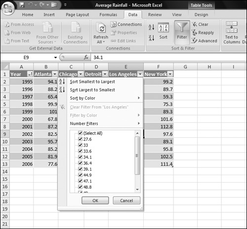
3.	To filter by an entry in a field, click the column’s AutoFilter drop-down arrow, and then click the to check the entry to match. Figure 19-16 shows an AutoFilter drop-down menu. If needed, you can click the Select All choice to clear all the checks, and then click a single check box to filter by that value. Figure 19-16. AutoFiltering. [View full size image]
4.	To create a more general filter, click the Number Filters choice, click one of the choices in the submenu that appears (Figure 19-17), specify the filter criteria in the Custom AutoFilter dialog box that appears (Figure 19-18), and then click OK to apply the filter. The field name appears in the dialog box, with the comparison operator you selected from the submenu already specified, as well. You can either select a value from the drop-down list on the right or type in a value of your own. Figure 19-17. This submenu offers choices for creating a custom AutoFilter. [View full size image] Figure 19-18. Specify the Custom AutoFilter criteria here.
5.	Specify another criterion if desired. When you add a second criterion for filtering, you have the option of using either a logical And or logical Or. With And, both criteria must be true; with Or, either criterion can be true. Click either the And or the Or radio button to select it.
6.	Click OK to implement the filtering.

To remove the filtering so that all the rows are visible, either select Clear Filters From from the drop-down-menus of each filtered field or select Data Sort & Filter Clear in the Ribbon. To turn off AutoFilter, select Data Sort & Filter Filter from the Ribbon.

Subtotaling data

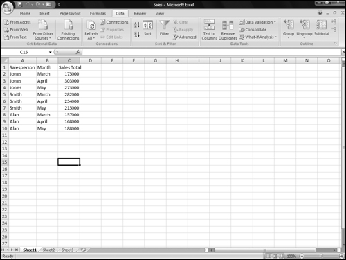
Excel’s subtotal feature is accessed via the Data tab of the Ribbon and is used with a sorted list. It’s not useful for every single type of database you can create, but only for those in which values can be kept track of for specific, repeated factors. Figure 19-19, for example, shows a database of sales people, which includes their monthly sales totals.

To subtotal a database, such as subtotaling the sales totals in this example by salesperson, follow these steps:

1.	Sort the database or table by the field you want to subtotal. In this case, that would be the Salesperson field.
2.	Select any cell within the database or table.
3.	Select Data Outline Subtotal from the Ribbon.
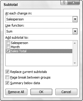
4.	In the Subtotal dialog box, click the drop-down list labeled At Each Change In and select the field that you want to subtotal, as shown in the example in Figure 19-20. Figure 19-20. Set up the subtotaling here.
5.	Select a function from the Use Function drop-down list. The functions listed in the drop-down list are the names of worksheet functions, some of which you learned about in earlier chapters. The available functions are as follows: Sum Count Average Max Min Product Count Numbers StdDev StdDevp Var Varp
6.	Select the fields for which you want to show subtotals in the Add Subtotal To area.
7.	Click the OK button. The subtotals appear in the list or table, as in the example shown in Figure 19-21. Figure 19-21. Database with subtotals added. [View full size image]

You can shrink the database so that only the subtotals show by clicking the minus signs to the left of the records.

To remove the subtotals, you can either click the Undo button immediately after adding the subtotals or select Data Outline Subtotal from the Ribbon, and then click the Remove All button.